2021-07-18 ce9206e22a233f02b45bae16d7714ee3 99+ 11 m 1.7 k

分类任务的衡量指标

一、二分类

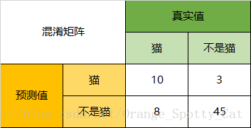
1.1 confusion matrix

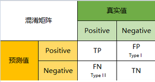
1.2 accuracy

$accuracy={\frac{TP+TN}{TP+TN+FP+FN}}$

accuracy 衡量全局分类正确的数量占总样本的比例

1.3 precision

$precision={\frac{TP}{TP+FP}}$

precision为预测正确正样本数占预测的全部正样本数的比例，即系统判定为正样本的正确率。通俗地说，假如医生给病人检查，医生判断病人有疾病，然后医生判断的正确率有多少。

1.4 recall

$recall={\frac{TP}{TP+FN}}$

recall为预测正确的正样本数量占真实正样本数量的比例，即衡量正样本的召回比例。通俗说，假如有一批病人，医生能从中找出病人的比例

1.5 F1

由于precision和recall往往是矛盾的，因此为了综合考虑二者，引入F1，即为precision和recall的调和平均

$F_{1}={2\frac{precision\cdot recall}{precision+recall}}$

当$precision$和$recall$的任一个值为0，$F_1$都为0

之所以采用调和平均，是因为调和平均数受极端值影响较大，更适合评价不平衡数据的分类问题

通用的F值表达式：

$F_{\beta}={(1+\beta^2)\frac{precision\cdot recall}{\beta^2\cdot precision+recall}}$

除了$F_1$分数之外，$F_2$ 分数和$F_{0.5}$分数在统计学中也得到大量的应用。其中，$F_2$分数中，召回率的权重高于精确率，而$F_{0.5}$分数中，精确率的权重高于召回率。

1.6 ROC

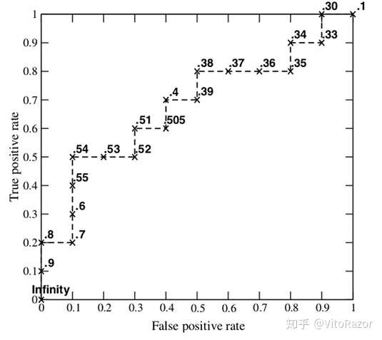
roc曲线：接收者操作特征(receiver operating characteristic), roc曲线上每个点反映某个阈值下的FPR和TPR的组合。

横轴：$FPR$，叫做假正类率，表示预测为正例但真实情况为反例的占所有真实情况中反例的比率，公式为$FPR=\frac{FP}{TN+FP}$。

纵轴：$TPR$ ，叫做真正例率，表示预测为正例且真实情况为正例的占所有真实情况中正例的比率，公式为

$TPR=\frac{TP}{TP+FN}$。

1.7 AUC

$AUC$(Area under Curve)：ROC曲线下的面积，数值可以直观评价分类器的好坏，值越大越好，对于二分类，结果介于0.5和1之间，1为完美分类器，0.5是因为二分类分类效果最差也是0.5。

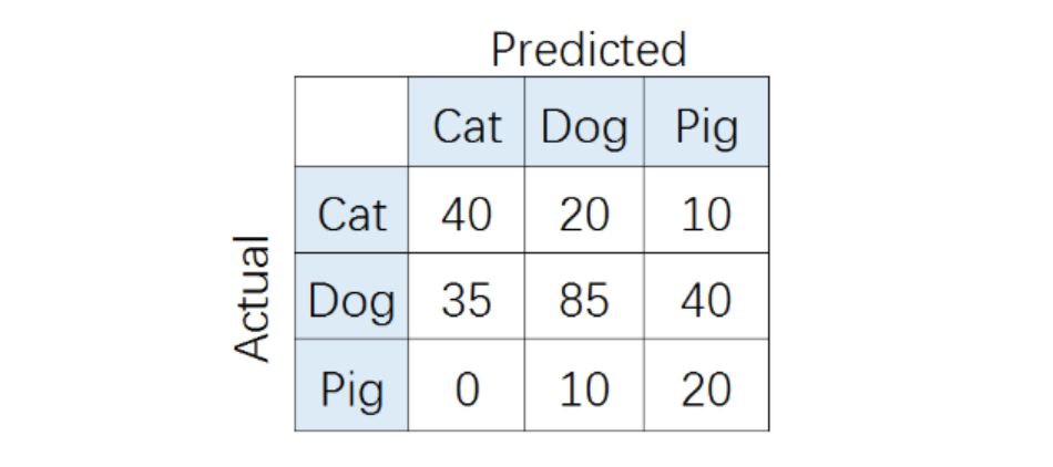
二、多分类

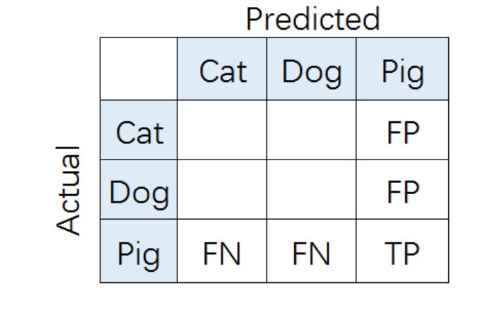
2.1 混淆矩阵

2.2 accuracy

$accuracy=\frac{分类正确的样本数,即对角线上的数}{总样本数，即矩阵全部元素相加}$

2.3 某个类别的precision，recall，F1

与二分类公式一样

$precision_{pig}=\frac{20}{20+(10+40)}=\frac{2}{7} \\recall_{pig}=\frac{20}{20+10}=\frac{2}{3} \\F_{1pig}={2\frac{precision_{pig}\cdot recall_{pig}}{precision_{pig}+recall_{pig}}}$

2.4 系统的precision，recall，F1

系统的precision，recall，$F_1$需要综合考虑所有类别，即同时考虑猫、狗、猪的precision，recall，$F_1$。有如下几种方案：

2.4.1 Macro average

$Macro-precision=\frac{precision_{cat}+precision_{dog}+precision_{pig}}{3} \\Macro-recall=\frac{recall{cat}+recall{dog}+recall{pig}}{3} \\Macro-F_{1}=\frac{F_{1cat}+F_{1dog}+F_{1pig}}{3}$

2.4.2 Weighted average

对macro的推广

$Weighted-precision=W_{cat}\cdot precision_{cat}+W_{dog}\cdot precision_{dog}+W_{pig}\cdot precision_{pig} \\Weighted-recall=W_{cat}\cdot recall{cat}+W_{dog}\cdot recall{dog}+W_{pig}\cdot recall{pig} \\Weighted-F_{1}=W_{cat}\cdot F_{1cat}+W_{dog}\cdot F_{1dog}+W_{pig}\cdot F_{1pig} \\W_{cat}:W_{dog}:W_{pig}=N_{cat}:N_{dog}:N_{pig},其中N为样本数量，W为权重$

2.4.3 Micro average

$Micro-precision={\frac{TP_{总}}{TP_{总}+FP_{总}}}={\frac{\sum_{i=1}^{n}TP_{i}}{\sum_{i=1}^{n}TP_{i}+\sum_{i=1}^{n}FP_{i}}} \\Micro-recall={\frac{TP_{总}}{TP_{总}+FN_{总}}}={\frac{\sum_{i=1}^{n}TP_{i}}{\sum_{i=1}^{n}TP_{i}+\sum_{i=1}^{n}FN_{i}}} \\Micro-F_{1}={2\frac{Micro-precision\cdot Micro-recall}{Micro-precision+Micro-recall}}$

2.5 ROC

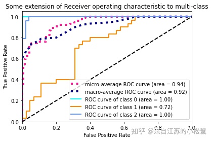
对于多分类分类器整体效果的ROC如上micro或者macro曲线，其余3条描述单个类别的分类效果。对于多分类，ROC上的点，同样是某个阈值下的FPR和TPR的组合。

对于多分类的$FPR$,$TPR$，有几种计算方式

a. micro average

$FPR_{micro } =\frac{FP_总}{TN_总+FP_总}=\frac{\sum_{i=1}^{n}FP_{i}}{\sum_{i=1}^{n}TN_{i}+\sum_{i=1}^{n}FP_{i}}\\ TPR_{micro }=\frac{TP_总}{TP_总+FN_总}=\frac{\sum_{i=1}^{n}TP_{i}}{\sum_{i=1}^{n}TP_{i}+\sum_{i=1}^{n}FN_{i}} \\n表示类别数量，FP_i，TN_i，TP_i，FN_i为某个类别的FP，TN，TP，FN$

b. macro average

$FPR_{macro}=\frac{1}{n}\sum_{i=1}^{n}FPR_{i}\\ TPR_{macro}=\frac{1}{n}\sum_{i=1}^{n}TPR_{i}，其中FPR_i，TPR_i为某个类别的FPR和TPR$

2.6 AUC

$AUC$依旧为ROC曲线下的面积，对于多分类个人认为取值范围为[0,1]。

三.代码

accuracy，precision，recall，F1

from sklearn.metrics import precision_recall_fscore_support, accuracy_score
def eval_acc_f1(y_true, y_pred):
    acc = accuracy_score(y_true, y_pred)
    prf = precision_recall_fscore_support(y_true, y_pred, average="macro")
    return acc, prf

ROC和AUC

# 引入必要的库
import numpy as np
import matplotlib.pyplot as plt
from itertools import cycle
from sklearn import svm, datasets
from sklearn.metrics import roc_curve, auc
from sklearn.model_selection import train_test_split
from sklearn.preprocessing import label_binarize
from sklearn.multiclass import OneVsRestClassifier
from scipy import interp

# 加载数据
iris = datasets.load_iris()
X = iris.data
y = iris.target
# 将标签二值化
y = label_binarize(y, classes=[0, 1, 2])
# 设置种类
n_classes = y.shape[1]

# 训练模型并预测
random_state = np.random.RandomState(0)
n_samples, n_features = X.shape

# shuffle and split training and test sets
X_train, X_test, y_train, y_test = train_test_split(X, y, test_size=.5,random_state=0)

# Learn to predict each class against the other
classifier = OneVsRestClassifier(svm.SVC(kernel='linear', probability=True,
                                 random_state=random_state))
y_score = classifier.fit(X_train, y_train).decision_function(X_test)

# 计算每一类的ROC
fpr = dict()
tpr = dict()
roc_auc = dict()
for i in range(n_classes):
    fpr[i], tpr[i], _ = roc_curve(y_test[:, i], y_score[:, i])
    roc_auc[i] = auc(fpr[i], tpr[i])

# Compute micro-average ROC curve and ROC area（方法二）
fpr["micro"], tpr["micro"], _ = roc_curve(y_test.ravel(), y_score.ravel())
roc_auc["micro"] = auc(fpr["micro"], tpr["micro"])

# Compute macro-average ROC curve and ROC area（方法一）
# First aggregate all false positive rates
all_fpr = np.unique(np.concatenate([fpr[i] for i in range(n_classes)]))
# Then interpolate all ROC curves at this points
mean_tpr = np.zeros_like(all_fpr)
for i in range(n_classes):
    mean_tpr += interp(all_fpr, fpr[i], tpr[i])
# Finally average it and compute AUC
mean_tpr /= n_classes
fpr["macro"] = all_fpr
tpr["macro"] = mean_tpr
roc_auc["macro"] = auc(fpr["macro"], tpr["macro"])

# Plot all ROC curves
lw=2
plt.figure()
plt.plot(fpr["micro"], tpr["micro"],
         label='micro-average ROC curve (area = {0:0.2f})'
               ''.format(roc_auc["micro"]),
         color='deeppink', linestyle=':', linewidth=4)

plt.plot(fpr["macro"], tpr["macro"],
         label='macro-average ROC curve (area = {0:0.2f})'
               ''.format(roc_auc["macro"]),
         color='navy', linestyle=':', linewidth=4)

colors = cycle(['aqua', 'darkorange', 'cornflowerblue'])
for i, color in zip(range(n_classes), colors):
    plt.plot(fpr[i], tpr[i], color=color, lw=lw,
             label='ROC curve of class {0} (area = {1:0.2f})'
             ''.format(i, roc_auc[i]))

plt.plot([0, 1], [0, 1], 'k--', lw=lw)
plt.xlim([0.0, 1.0])
plt.ylim([0.0, 1.05])
plt.xlabel('False Positive Rate')
plt.ylabel('True Positive Rate')
plt.title('Some extension of Receiver operating characteristic to multi-class')
plt.legend(loc="lower right")
plt.show()