Enhanced-RCNN An Efficient Method for Learning Sentence Similarity

特点:非预训练,参数量少

1 input encoding

得到两个encoding,RNN Encoding,RCNN Encoding

1 BiGRU

$\textbf{a}=\{a_1,a_2,…,a_{l_a}\},\textbf{a}$ 是句子,$l_a$ 是句子1的长度

得到RNN Encoding,$\overline{\textbf{p}}_i$统一表示$\overline{\textbf{a}}_i,\overline{\textbf{b}}_i$

2 CNN

在 BiGRU 编码的基础上,使用 CNN 来进行二次编码

结构如下,“newtork in network”,k 是卷积核的kernel size,比如k=1,卷积核为$1 \times 1$

对于每个 CNN 单元,具体的计算过程如下:

得到 RCNN Encoding $\widetilde{\textbf{p}}_i$

2 Interactive Sentence Representation

1 Soft-attention Alignment

attention:

加了attention的rnn encoding:

2 Interaction Modeling

$\overline{\textbf{p}}$是rnn encoding

$\hat{}$是加了attention的rnn encoding

$\widetilde{}$是rcnn encoding

最终得到Interactive Sentence Representation为$\textbf{o}_a,\textbf{o}_b$

3 Similarity Modeling

1 Fusion Layer

g是门控函数

2 Label Prediction

全连接层

4 loss

交叉熵

参考

https://sci-hub.st/10.1145/3366423.3379998

https://zhuanlan.zhihu.com/p/138061003

Bridging the Gap Between Relevance Matching and Semantic Matching for Short Text Similarity Modeling

https://cs.uwaterloo.ca/~jimmylin/publications/Rao_etal_EMNLP2019.pdf

2 HCAN: Hybrid Co-Attention Network

three major components: (1) a hybrid encoder (2) a relevance matching module (3) a semantic matching module

2.1 Hybrid Encoders

hybrid encoder module that explores three types of encoders: deep, wide, and contextual

query and context words :$\{w_1^q,w_2^q,…,w_n^q\},\{w_1^c,w_2^c,…,w_m^c\}$, embedding representations $\textbf{Q}\in \mathbb{R}^{n\times L},\textbf{C}\in \mathbb{R}^{m\times L}$

Deep Encoder

$\textbf{U}$表示$\textbf{Q},\textbf{C}$

Wide Encoder

Unlike the deep encoder that stacks multiple convolutional layers hierarchically, the wide encoder organizes convolutional layers in parallel, with each convolutional layer having a different window size k

Contextual Encoder

2.2 Relevance Matching

2.3 Semantic Matching

2.4 Final Classification

文本匹配

1.无监督

1.1 编辑距离

定义

编辑距离,英文名字为Levenshtein distance,通过描述一个字符串A需要多少次基本操作可以变成字符串B,来衡量两个字符串的相似度。

基本操作包括:增、删、改

增:字符串A为“AS”,字符串B为“ ASD“,字符串A->字符串B需要增加一个字符“D”

删:字符串A为“ASD”,字符串B为“ AS“,字符串A->字符串B需要删除一个字符“D”

改:字符串A为“ASX”,字符串B为“ ASD“,字符串A->字符串B需要将字符“X”变成字符“D”

代码

实现过程使用动态规划,递推公式为

$i$和$j$分别表示字符串$a$和字符串$b$的下标,$lev_{a,b}(i,j)$表示子串$a[:i]$到子串$b[:j]$的编辑距离。

1
2
3
4
5
6
7
8
9
10
11
12
13
14
15
16
17
18
19
20
21
22
23
24
def lev(str_a,str_b):
"""
ED距离,用来衡量单词之间的相似度
:param str_a:
:param str_b:
:return:
"""
str_a=str_a.lower()
str_b=str_b.lower()
matrix_ed=np.zeros((len(str_a)+1,len(str_b)+1),dtype=np.int)
matrix_ed[0]=np.arange(len(str_b)+1)
matrix_ed[:,0] = np.arange(len(str_a) + 1)
for i in range(1,len(str_a)+1):
for j in range(1,len(str_b)+1):
# 表示删除a_i
dist_1 = matrix_ed[i - 1, j] + 1
# 表示插入b_i
dist_2 = matrix_ed[i, j - 1] + 1
# 表示替换b_i
dist_3 = matrix_ed[i - 1, j - 1] + (1 if str_a[i - 1] != str_b[j - 1] else 0)
#取最小距离
matrix_ed[i,j]=np.min([dist_1, dist_2, dist_3])
print(matrix_ed)
return matrix_ed[-1,-1]

1.2 TF-IDF

原理

(1)TF

针对某个doc

越大,这个term在doc中越普通

$TF_{term}=\frac{term在doc中出现的次数}{doc所有词的总数}$

(2)IDF

针对所有doc

越大,这个term在doc集合中越稀有

$IDF_{term}=log(\frac{doc总数}{包含该term的doc数+1})$

(3)TF-IDF

综合上面

$TF-IDF_{term}=TF_{term}*IDF_{term}$

(4)TF-IDF VEC

现有句子A:”今天天气真好”,对句子A做分词得到[“今天”,”天气”,”真好”],词库包含[“今天”,”天气”,”真好”,”天气”,”不错呀”]

$VEC_{A}=[TF-IDF_{今天},TF-IDF_{天气},TF-IDF_{真好},0,0]$

(5)计算两句话的文本相似度

假设词库包含[“今天”,”天气”,”真好”,”天气”,”不错呀”],现有句子A:”今天天气真好”,对句子A做分词得到[“今天”,”天气”,”真好”],句子B:”天气不错呀”,分词后[“天气”,”不错呀”]

利用(3)得到句子A的TF-IDF VEC $VEC_{A}$,句子B的TF-IDF VEC $VEC_B$,利用余弦相似度计算文本相似度

代码

1
2
3
4
5
6
7
8
9
10
11
12
13
14
15
16
17
18
19
20
21
22
23
24
25
26
27
28
29
30
31
32
33
34
35
36
37
38
39
40
41
42
43
44
45
46
47
48
49
50
51
52
53
54
55
56
57
58
59
60
61
62
63
64
65
66
67
68
69
70
71
72
73
74
75
76
77
78
79
80
81
82
import pandas as pd
import jieba
import numpy as np
from sklearn.externals import joblib
from scipy.linalg import norm


class TF_IDF_Model(object):
def __init__(self, corpus_list):

self.documents_list = corpus_list
self.documents_number = len(corpus_list)
self.get_idf()

def get_idf(self):
df = {}
self.idf = {}
tf = []
for document in self.documents_list:
temp = {}
for word in document:
temp[word] = temp.get(word, 0) + 1 / len(document)
tf.append(temp)
for key in temp.keys():
df[key] = df.get(key, 0) + 1
for key, value in df.items():
self.idf[key] = np.log10(self.documents_number / (value + 1))

def get_tf(self, document):
document = list(jieba.cut(document))
# tf = []
temp = {}
for word in document:
temp[word] = temp.get(word, 0) + 1 / len(document)
# tf.append(temp)
return temp

def tf_idf_vec(self, text):
tf = self.get_tf(text)
word = list(self.idf.keys())
vec = [0] * len(self.idf)
text = list(jieba.cut(text))
for ele in text:
if ele in word:
vec[word.index(ele)] = tf[ele] * self.idf[ele]
return vec

def cal_similarty(self, sentence1, sentence2):
vec1 = self.tf_idf_vec(sentence1)
vec2 = self.tf_idf_vec(sentence2)
similarty = np.dot(vec1, vec2) / (norm(vec1) * norm(vec2))
return similarty


def train_model():
#####bulid corpus
corpus = pd.read_csv(corpus_path)
corpus_list = corpus["name"].get_values().tolist()
# corpus_list = corpus1["name"].get_values().tolist()
corpus_list = [list(jieba.cut(str(doc))) for doc in corpus_list]
tf_idf_model = TF_IDF_Model(corpus_list)
joblib.dump(tf_idf_model, model_path)


def load_model(path):
tf_idf_model = joblib.load(path)
return tf_idf_model


if __name__ == '__main__':
from supercat.data_qualifier.tf_idf import TF_IDF_Model
####
train_model()
######
tf_idf_model = load_model(model_path)
sentence1="XXXX"
sentence2="XXXX"
print(tf_idf_model.get_tf(sentence1))
print(tf_idf_model.idf)
print(tf_idf_model.tf_idf_vec(sentence1))
print(tf_idf_model.cal_similarty(sentence1,sentence2))

2.有监督

基于表示的匹配方法:使用深度学习模型分别表征Query和Doc,通过计算向量相似度来作为语义匹配分数。微软的DSSM[26]及其扩展模型属于基于表示的语义匹配方法,美团搜索借鉴DSSM的双塔结构思想,左边塔输入Query信息,右边塔输入POI、品类信息,生成Query和Doc的高阶文本相关性、高阶品类相关性特征,应用于排序模型中取得了很好的效果。此外,比较有代表性的表示匹配模型还有百度提出 SimNet[27],中科院提出的多视角循环神经网络匹配模型(MV-LSTM)[28]等。

基于交互的匹配方法:这种方法不直接学习Query和Doc的语义表示向量,而是在神经网络底层就让Query和Doc提前交互,从而获得更好的文本向量表示,最后通过一个MLP网络获得语义匹配分数。代表性模型有华为提出的基于卷积神经网络的匹配模型ARC-II[29],中科院提出的基于矩阵匹配的的层次化匹配模型MatchPyramid[30]。

基于表示的匹配方法优势在于Doc的语义向量可以离线预先计算,在线预测时只需要重新计算Query的语义向量,缺点是模型学习时Query和Doc两者没有任何交互,不能充分利用Query和Doc的细粒度匹配信号。基于交互的匹配方法优势在于Query和Doc在模型训练时能够进行充分的交互匹配,语义匹配效果好,缺点是部署上线成本较高。

匹配不同于排序,匹配是1对1的,排序是1对多

2.1基于表示

https://zhuanlan.zhihu.com/p/138864580

https://blog.csdn.net/qq_27590277/article/details/121391770

2.2.基于交互

https://blog.csdn.net/guofei_fly/article/details/107501276

Neural Graph Matching Networks for Chinese Short Text Matching

https://aclanthology.org/2020.acl-main.547.pdf

1.摘要

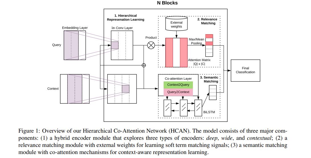
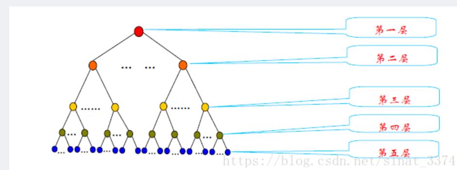
对于中文短文本匹配,通常基于词粒度而不是字粒度。但是分词结果可能是错误的、模糊的或不一致的,从而损害最终的匹配性能。比如下图:字符序列“南京市长江大桥”经过不同的分词可能表达为不同的意思。

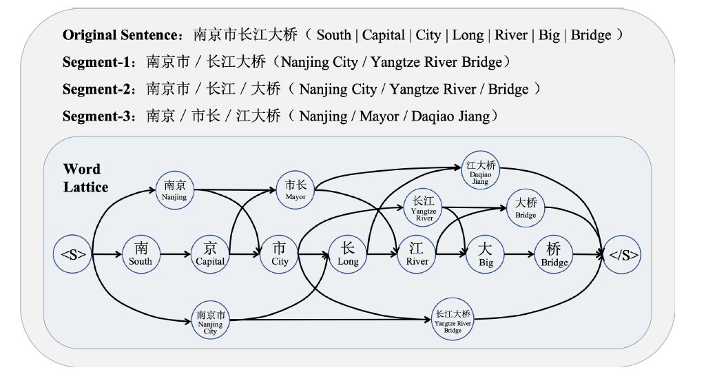
为了解决这个问题,作者提出了一种基于图神经网络的中文短文本匹配方法。不是将句子分割成一个单词序列,而是保留所有可能的分割路径,形成一个Lattice(segment1,segment2,segment3),如上图所示。

2.问题定义

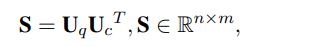
将两个待匹配中文短文本分别定义为$S_a=\left \{ C_1^a,C_2^a,…,C_{t_a}^a \right \}$,$S_b=\left \{ C_1^b,C_2^b,…,C_{t_b}^b \right \}$,其中$C_i^a$表示句子$a$第$i$个字,$C_j^b$表示句子$b$第$j$个字,$t_a$,$t_b$分别表示两个句子的长度。$f(S_a,S_b)$是目标函数,输出为两个文本的匹配度。词格图用$G=(\nu,\xi)$表示,其中$\nu$是节点集,包括所有字符序列。$\xi$表示边集,如果$\nu$中两个顶点$v_i$和$v_j$相邻,那么就存在一个边为$e_{ij}$。$N_{fw}(v_i)$表示节点$v_i$ 正向的所有可达节点的集合,$N_{bw}(v_i)$表示节点$v_i$ 反向的所有可达节点的集合。句子$a$的词格图为$G^a(\nu_a,\xi_a)$,句子$b$的词格图为$G^b(\nu_b,\xi_b)$。

3.模型结构

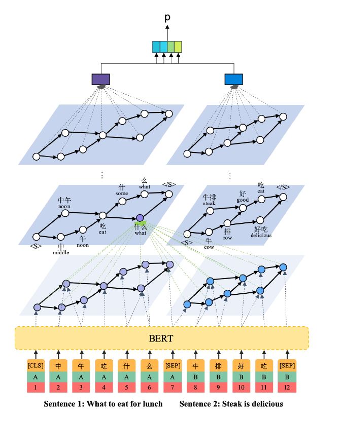
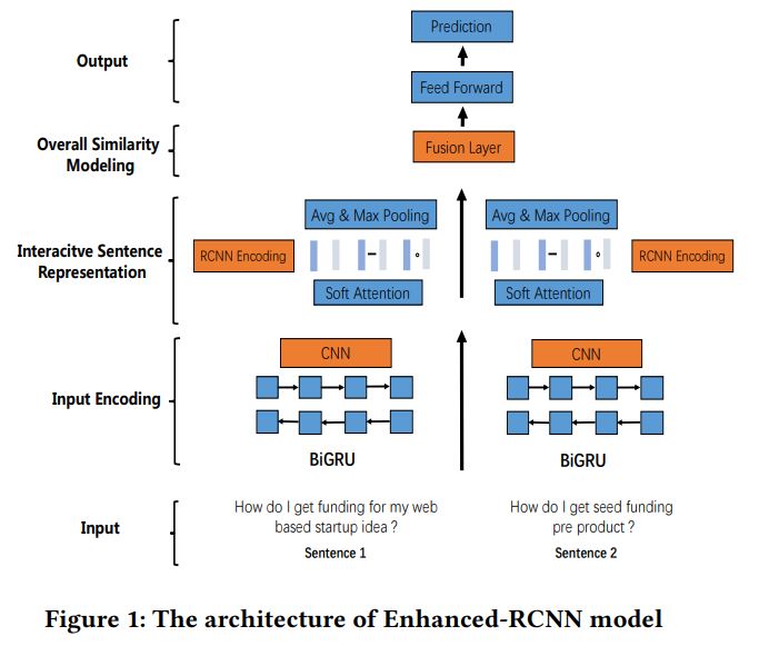
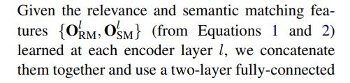
模型分成3个部分,1.语言节点表示 2.图神经匹配 3.相关性分类器

3.1 语言节点表示

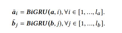
这一部分基于BERT的结构。BERT的token表示基于字粒度,可以得到$\left \{ [CLS],C_1^a,C_2^a,…,C_{ta}^a,[SEP],C_1^b,C_2^b,…,C_{t_b}^b,[SEP] \right \}$,如上图所示。BERT的输出为各个字的Embedding,$ \left \{\textbf{C}^{CLS},\textbf{C}_1^a,\textbf{C}_2^a,…,\textbf{C}_{t_a}^a,\textbf{C}^{SEP},\textbf{C}_1^b,\textbf{C}_2^b,…,\textbf{C}_{t_b},\textbf{C}^{SEP} \right \}$。
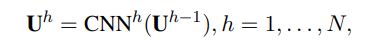
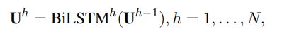
3.2 图神经匹配

初始化:假设节点$v_i$包含$n_i$个连续字符,起始字符位置为$s_i$,即$ \left \{C_{s_i},C_{s_{i+1}},…,C_{s_{i}+n_i-1} \right \}$,这里$v_i$表示句子$a$或者$b$的结点。$V_i=\sum_{k=0}^{n_i-1}\textbf{U}_{s_i+k}\odot\textbf{C}_{s_i+k}$,其中$\odot$表示两个向量对应各个元素相乘。特征识别分数向量$\textbf{U}_{s_i+k}=softmax(FFN(\textbf{C}_{s_i+k}))$,$FFN$为两层。$h$为结点的向量表示,将$h_i^0$等于$V_i$

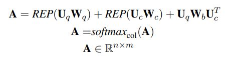
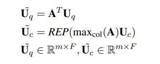
Message Propagation : 对于第$l$次迭代,$G_a$中某个结点$v_i$由如下四个部分组成

其中$\alpha_{ij},\alpha_{ik},\alpha_{im},\alpha_{iq}$是注意力系数,$W^{fw},W^{bw}$是注意力系数参数

然后定义两种信息为$m_i^{self}\triangleq[m_i^{fw},m_i^{bw}],m_i^{cross}\triangleq[m_i^{b1},m_i^{b2}]$

Representation Updating:得到两种信息后,需要更新结点$ v_i$的向量表示

其中$w_k^{cos}$为参数,$d_k$为multi-perspective cosine distance,可以衡量两种信息的距离,$k \in \left \{ 1,2,3,…P\right\}$,$P$是视角的数量。

其中$\textbf{d}_i\triangleq[d_1,d_2,…,d_P]$,$FFN$两层。

句子的图级别表示

总共经历了$L$次迭代(layer),得到$h_i^L$为结点$v_i$最终的向量表示($h_i^L$includes not only the information from its reachable nodes but also information of pairwise comparison with all nodes in another graph)
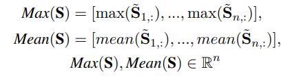
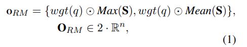
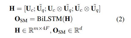
最终,两个句子的图级别表示分别为

3.3 分类器

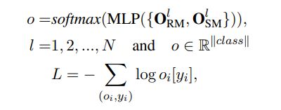
得到$g^a,g^b$后,两句子的相似度可以用分类器衡量:

其中$P \in [0,1]$。

4.实验结果

lattice和JIEBA+PKU的区别?

JIEBA+PKU is a small lattice graph generated by merging two word segmentation results

lattice:overall lattice,应该是全部的组合

两者效果差不多是因为Compared with the tiny graph, the overall lattice has more noisy nodes (i.e. invalid words in the corresponding sentence).

参考

https://blog.csdn.net/qq_43390809/article/details/114077216

词语的文本相似度

一.基于词典

人为构建,比较主观,不利于维护

1.1 基于词林

1.1.1 结构

扩展版同义词词林分为5层结构,如图,随着级别的递增,词义刻画越来越细,到了第五层,每个分类里词语数量已经不大,很多只有一个词语,已经不可再分,可以称为原子词群、原子类或原子节点。不同级别的分类结果可以为自然语言处理提供不同的服务,例如第四层的分类和第五层的分类在信息检索、文本分类、自动问答等研究领域得到应用。有研究证明,对词义进行有效扩展,或者对关键词做同义词替换可以明显改善信息检索、文本分类和自动问答系统的性能。

下载后的词典文件如下所示:

1
2
3
4
5
Aa01A01= 人 士 人物 人士 人氏 人选
Aa01A02= 人类 生人 全人类
Aa01A03= 人手 人员 人口 人丁 口 食指
Aa01A04= 劳力 劳动力 工作者
Aa01A05= 匹夫 个人

表中的编码位是按照从左到右的顺序排列。第八位的标记有3 种,分别是“=”、“#”、“@”, “=”代表“相等”、“同义”。末尾的“#”代表“不等”、“同类”,属于相关词语。末尾的“@”代表“自我封闭”、“独立”,它在词典中既没有同义词,也没有相关词。

源码如下

1
2
3
4
5
6
7
8
9
10
11
12
13
14
15
16
17
18
19
20
21
22
23
24
25
26
27
28
29
30
31
32
33
34
35
36
37
38
39
40
41
42
43
44
45
46
47
48
49
50
51
52
53
54
55
56
57
58
59
60
61
62
63
64
65
66
67
68
69
70
71
72
73
74
75
76
77
78
79
80
81
82
83
84
85
86
87
88
89
90
91
92
93
94
95
96
97
98
99
100
101
102
103
104
105
106
107
108
109
110
111
112
113
114
115
116
117
118
119
120
121
122
123
124
125
126
127
128
129
130
131
132
133
class WordSimilarity2010(SimilarBase):
'''
本类根据下面的论文方法:
基于同义词词林的词语相似度计算方法,田久乐, 赵 蔚(东北师范大学 计算机科学与信息技术学院, 长春 130117 )
计算两个单词所有编码组合的相似度,取最大的一个
'''

def __init__(self):
super(WordSimilarity2010, self).__init__()
self.a = 0.65
self.b = 0.8
self.c = 0.9
self.d = 0.96
self.e = 0.5
self.f = 0.1
self.degree = 180
self.PI = math.pi

def similarity(self, w1, w2):
'''
判断两个词的相似性。
:param w1: [string]
:param w2: [string]
:return: [float]0~1之间。
'''

code1 = self._data.get(w1, None)
code2 = self._data.get(w2, None)

if not code1 or not code2:
return 0 # 只要有一个不在库里则代表没有相似性。

# 最终返回的最大相似度
sim_max = 0

# 两个词可能对应多个编码
for c1 in code1:
for c2 in code2:
cur_sim = self.sim_by_code(c1, c2)
# print(c1, c2, '的相似度为:', cur_sim)
if cur_sim > sim_max:
sim_max = cur_sim

return sim_max

def sim_by_code(self, c1, c2):
"""
根据编码计算相似度
"""

# 先把code的层级信息提取出来
clayer1 = self._parse_code(c1)
clayer2 = self._parse_code(c2)

common_layer = self.get_common_layer(clayer1,clayer2)
length = len(common_layer)

# 如果有一个编码以'@'结尾,那么表示自我封闭,这个编码中只有一个词,直接返回f
if c1.endswith('@') or c2.endswith('@') or 0 == length:
return self.f

cur_sim = 0
if 6 <= length:
# 如果前面七个字符相同,则第八个字符也相同,要么同为'=',要么同为'#''
if c1.endswith('=') and c2.endswith('='):
cur_sim = 1
elif c1.endswith('#') and c2.endswith('#'):
cur_sim = self.e
else:
k = self.get_k(clayer1, clayer2)
n = self.get_n(common_layer)
if 1 == length:
cur_sim = self.sim_formula(self.a, n, k)
elif 2 == length:
cur_sim = self.sim_formula(self.b, n, k)
elif 3 == length:
cur_sim = self.sim_formula(self.c, n, k)
elif 4 == length:
cur_sim = self.sim_formula(self.d, n, k)

return cur_sim

def sim_formula(self, coeff, n, k):
"""
计算相似度的公式,不同的层系数不同
"""
return coeff * math.cos(n * self.PI / self.degree) * ((n - k + 1) / n)

def get_common_layer(self, ca, cb):
'''
返回相应的layer层
:param ca: [list(str)] 分解后的编码。
:param cb: [list(str)] 分解后的编码。
:return: [list(str)]列表代表相应的根编码。
'''
common_layer = []

for i, j in zip(ca, cb):
if i == j:
common_layer.append(i)
else:
break
return common_layer

def get_k(self, c1, c2):
"""
返回两个编码对应分支的距离,相邻距离为1
"""
if c1[0] != c2[0]:
return abs(ord(c1[0]) - ord(c2[0]))
elif c1[1] != c2[1]:
return abs(ord(c1[1]) - ord(c2[1]))
elif c1[2] != c2[2]:
return abs(int(c1[2]) - int(c2[2]))
elif c1[3] != c2[3]:
return abs(ord(c1[3]) - ord(c2[3]))
else:
return abs(int(c1[4]) - int(c2[4]))

def get_n(self, common_layer):
'''
返回相应结点下有多少个同级子结点。
:param common_layer: [listr(str)]相同的结点。
:return: int
'''

end_node = self._code_tree
for t_node_name in common_layer:
end_node = end_node[t_node_name]

if not isinstance(end_node, dict):
return end_node
return len(end_node.keys())

1.1.2 使用

环境准备:pip install WordSimilarity

1
2
3
4
5
6
7
8
9
10
11
12
13
14
15
16
17
from word_similarity import WordSimilarity2010
import time

ws_tool = WordSimilarity2010()
start = time.time()
b_a = "联系方式"
b_b = "电话"
sim_b = ws_tool.similarity(b_a, b_b)
print(b_a, b_b, '相似度为', sim_b)
end = time.time()
print("运行时间:"+str(end-start))
b_a = "手机"
b_b = "电话"
sim_b = ws_tool.similarity(b_a, b_b)
print(b_a, b_b, '相似度为', sim_b)
end = time.time()
print("运行时间:"+str(end-start))
1
2
3
4
联系方式 电话 相似度为 0
运行时间:5.793571472167969e-05
手机 电话 相似度为 0.30484094213212237
运行时间:0.0001442432403564453

1.2 基于知网与词林的词语语义相似度计算

1.2.1 原理

综合了词林cilin与知网hownet的相似度计算方法,采用混合策略,混合策略具体可以参考源码,如下

1
2
3
4
5
6
7
8
9
10
11
12
13
14
15
16
17
18
19
20
21
22
23
24
25
26
27
28
29
30
31
32
33
34
35
36
37
38
39
40
41
42
43
44
45
46
47
48
49
50
51
52
53
54
55
56
57
58
59
60
61
62
63
64
65
66
67
68
69
70
71
72
73
74
75
76
77
78
79
80
81
82
83
84
85
from hownet.howNet import How_Similarity
from cilin.V3.ciLin import CilinSimilarity

class HybridSim():
'''
混合相似度计算策略。使用了词林与知网词汇量的并集。扩大了词汇覆盖范围。
'''
ci_lin = CilinSimilarity() # 实例化词林相似度计算对象
how_net = How_Similarity() # 实例化知网相似度计算对象
Common = ci_lin.vocab & how_net.vocab
A = how_net.vocab - ci_lin.vocab
B = ci_lin.vocab - how_net.vocab

@classmethod
def get_Final_sim(cls, w1, w2):
lin = cls.ci_lin.sim2018(w1, w2) if w1 in cls.ci_lin.vocab and w2 in cls.ci_lin.vocab else 0
how = cls.how_net.calc(w1, w2) if w1 in cls.how_net.vocab and w2 in cls.how_net.vocab else 0

if w1 in cls.Common and w2 in cls.Common: # 两个词都被词林和知网共同收录。
# print('两个词都被词林和知网共同收录。', end='\t')
# print(w1, w2, '词林改进版相似度:', lin, end='\t')
# print('知网相似度结果为:', how, end='\t')
return lin * 1 + how * 0 # 可以调节两者的权重,以获取更优结果!!

if w1 in cls.A and w2 in cls.A: # 两个词都只被知网收录。
return how
if w1 in cls.B and w2 in cls.B: # 两个词都只被词林收录。
return lin

if w1 in cls.A and w2 in cls.B: # 一个只被词林收录,另一个只被知网收录。
print('触发策略三,左词为知网,右词为词林')
same_words = cls.ci_lin.code_word[cls.ci_lin.word_code[w2][0]]
if not same_words:
return 0.2
all_sims = [cls.how_net.calc(word, w1) for word in same_words]
print(same_words, all_sims, end='\t')
return max(all_sims)

if w2 in cls.A and w1 in cls.B:
print('触发策略三,左词为词林,右词为知网')
same_words = cls.ci_lin.code_word[cls.ci_lin.word_code[w1][0]]
if not same_words:
return 0.2
all_sims = [cls.how_net.calc(word, w2) for word in same_words]
print(w1, '词林同义词有:', same_words, all_sims, end='\t')
return max(all_sims)

if w1 in cls.A and w2 in cls.Common:
print('策略四(左知网):知网相似度结果为:', how)
same_words = cls.ci_lin.code_word[cls.ci_lin.word_code[w2][0]]
if not same_words:
return how
all_sims = [cls.how_net.calc(word, w1) for word in same_words]
print(w2, '词林同义词有:', same_words, all_sims, end='\t')
return 0.6 * how + 0.4 * max(all_sims)

if w2 in cls.A and w1 in cls.Common:
print('策略四(右知网):知网相似度结果为:', how)
same_words = cls.ci_lin.code_word[cls.ci_lin.word_code[w1][0]]
if not same_words:
return how
all_sims = [cls.how_net.calc(word, w2) for word in same_words]
print(same_words, all_sims, end='\t')
return 0.6 * how + 0.4 * max(all_sims)

if w1 in cls.B and w2 in cls.Common:
print(w1, w2, '策略五(左词林):词林改进版相似度:', lin)
same_words = cls.ci_lin.code_word[cls.ci_lin.word_code[w1][0]]
if not same_words:
return lin
all_sims = [cls.how_net.calc(word, w2) for word in same_words]
print(w1, '词林同义词有:', same_words, all_sims, end='\t')
return 0.6 * lin + 0.4 * max(all_sims)

if w2 in cls.B and w1 in cls.Common:
print(w1, w2, '策略五(右词林):词林改进版相似度:', lin)
same_words = cls.ci_lin.code_word[cls.ci_lin.word_code[w2][0]]
if not same_words:
return lin
all_sims = [cls.how_net.calc(word, w1) for word in same_words]
print(w2, '词林同义词有:', same_words, all_sims, end='\t')
return 0.6 * lin + 0.4 * max(all_sims)

print('对不起,词语可能未收录,无法计算相似度!')
return -1

1.2.2 使用

参考https://github.com/yaleimeng/Final_word_Similarity

1
2
3
4
5
6
7
8
9
10
11
12
13
14
15
16
17
18
19
20
21
22
23
24
25
from Hybrid_Sim import HybridSim
from Pearson import *

import time


if __name__ == '__main__':

print('词林词汇量', len(HybridSim.ci_lin.vocab ),'\t知网词汇量', len(HybridSim.how_net.vocab))
print('两者总词汇量',len(HybridSim.ci_lin.vocab | HybridSim.how_net.vocab),'\t重叠词汇量', len(HybridSim.Common))
b_a = "联系方式"
b_b = "电话"
start = time.time()
hybrid = HybridSim.get_Final_sim(b_a, b_a)
end = time.time()
print(b_a+" "+b_b+"相似度为:", hybrid)
print("运行时间:"+str(end-start))
b_a = "手机"
b_b = "电话"
start = time.time()
hybrid = HybridSim.get_Final_sim(b_a, b_a)
end = time.time()
print(b_a+" "+b_b+"相似度为:", hybrid)
print("运行时间:"+str(end-start))

1
2
3
4
5
6
7
词林词汇量 77498 	知网词汇量 53336
两者总词汇量 85817 重叠词汇量 45017
对不起,词语可能未收录,无法计算相似度!
联系方式 电话相似度为: -1
运行时间:3.504753112792969e-05
手机 电话相似度为: 1.0
运行时间:0.019332408905029297

二.基于词向量

基于样本构建,利于维护

2.1 基于word2vec

2.2.1 原理

word2vec的原理和词向量获取过程不在此赘述,在本部分主要讲解基于word2vec的词向量如何计算词语相似度。源码如下

1
2
3
4
5
6
7
8
9
10
11
12
13
14
15
16
17
def similarity(self, w1, w2):
"""Compute cosine similarity between two keys.

Parameters
----------
w1 : str
Input key.
w2 : str
Input key.

Returns
-------
float
Cosine similarity between `w1` and `w2`.

"""
return dot(matutils.unitvec(self[w1]), matutils.unitvec(self[w2]))

2.2.2 使用

训练

1
2
3
4
5
6
7
8
9
10
11
from gensim.models.word2vec import Word2Vec
import pandas as pd
from gensim import models
import jieba
###train
data=pd.read_csv(data_path)
sentences=data.tolist()
model= Word2Vec()
model.build_vocab(sentences)
model.train(sentences,total_examples = model.corpus_count,epochs = 5)
model.save(model_path)

使用

1
2
3
4
5
6
7
8
9
10
11
12
13
14
15
16
17
18
19
from gensim import models
import time

if __name__ == '__main__':
model=models.Word2Vec.load(model_path)
start = time.time()
b_a = "联系方式"
b_b = "电话"
sim_b = model.wv.n_similarity(b_a, b_b)
end = time.time()
start = time.time()
print(b_a, b_b, '相似度为', sim_b)
print("运行时间:" + str(end - start))
b_a = "手机"
b_b = "电话"
sim_b = model.wv.n_similarity(b_a, b_b)
end = time.time()
print(b_a, b_b, '相似度为', sim_b)
print("运行时间:" + str(end - start))
1
2
3
4
联系方式 电话 相似度为 -0.014857853
运行时间:-4.76837158203125e-07
手机 电话 相似度为 0.1771852
运行时间:0.0004227161407470703

参考文献

https://blog.csdn.net/sinat_33741547/article/details/80016713

https://github.com/yaleimeng/Final_word_Similarity


:D 一言句子获取中...