Evaluation of Text Generation A Survey

从3个维度将评价指标分类

1 Human-Centric Evaluation Methods

​ gold standard expensive to execute

2 Untrained Automatic Evaluation Metrics

widely used

汇总

property: 应该是说这个方法的关注点

3 Untrained Automatic Evaluation Metrics

over fitting and `gaming of the metric.’

参考

https://arxiv.org/abs/2006.14799

Felix Flexible Text Editing Through Tagging and Insertion

google继lasertagger之后的又一篇text edit paper

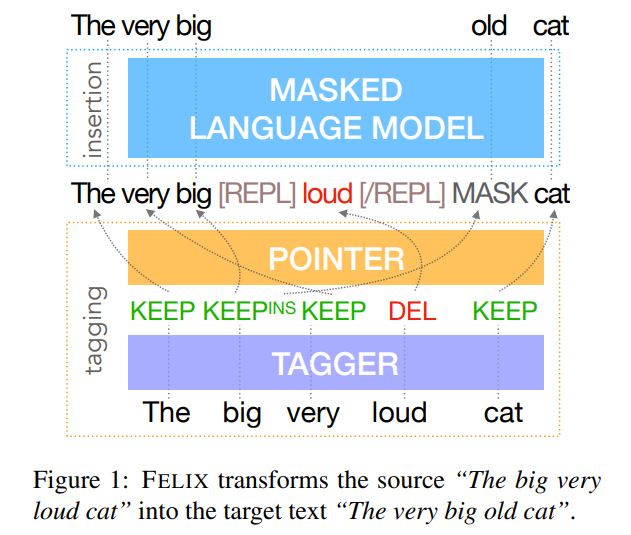
In contrast to conventional sequence-to-sequence (seq2seq) models, FELIX is efficient in low-resource settings and fast at inference time, while being capable of modeling flexible input-output transformations. We achieve this by decomposing the text-editing task into two sub-tasks: tagging to decide on the subset of input tokens and their order in the output text and insertion to in-fill the missing tokens in the output not present in the input.

1 Introduction

In particular, we have designed FELIX with the following requirements in mind: Sample efficiency, Fast inference time, Flexible text editing

2 Model description

FELIX decomposes the conditional probability of generating an output sequence $y$ from an input
$x$ as follows:

2.1 Tagging Model

trained to optimize both the tagging and pointing loss:

Tagging :

tag sequence $\textbf{y}^t$由3种tag组成:$KEEP$,$DELETE$,$INSERT (INS)$

Tags are predicted by applying a single feedforward layer $f$ to the output of the encoder $\textbf{h}^L$ (the source sentence is first encoded using a 12-layer BERT-base model). $\textbf{y}^t_i=argmax(f(\textbf{h}^L_i))$

Pointing:

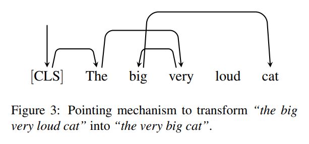
Given a sequence $\textbf{x}$ and the predicted tags $\textbf{y}^t$ , the re-ordering model generates a permutation $\pi$ so that from $\pi$and $\textbf{y}^t$ we can reconstruct the insertion model input $\textbf{y}^m$. Thus we have:

Our implementation is based on a pointer network. The output of this model is a series of predicted pointers (source token → next target token)

The input to the Pointer layer at position $i$:

其中$e(\textbf{y}_i^t)$is the embedding of the predicted tag,$e(\textbf{p}_i)$ is the positional embedding

The pointer network attends over all hidden states, as such:

其中$\textbf{h}_i^{L+1}$ as $Q $, $\textbf{h}_{\pi(i)}^{L+1}$ as $K$

When realizing the pointers, we use a constrained beam search

2.2 Insertion Model

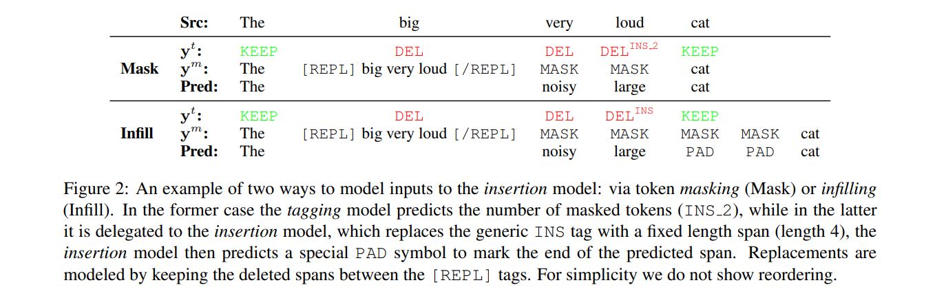
To represent masked token spans we consider two options: masking and infilling. In the former case the tagging model predicts how many tokens need to be inserted by specializing the $INSERT$ tag into $INS_k$, where $k$ translates the span into $ k$ $MASK$ tokens. For the infilling case the tagging model predicts a generic $INS$ tag.

Note that we preserve the deleted​ span in the input to the insertion model by enclosing it between $[REPL]$ and $[/REPL]$ tags.

our insertion model is also based on a 12-layer BERT-base and we can directly take advantage of the BERT-style pretrained checkpoints.

参考

https://aclanthology.org/2020.findings-emnlp.111.pdf

LASERTAGGER

一. 摘要

对于某一些文本生成任务,输入和输出的文本有很多的重叠部分,如果还是采用encoder-decoder的文本生成模型去从零开始生成,其实是很浪费和没必要的,并且会导致两个问题:1:生成模型的幻觉问题(就是模型胡说八道) ;2:出现叠词(部分片段一致)。

基于上面的考虑,作者提出了lasertagger模型,通过几个常用的操作:keep token、delete token、 add token,给输入序列的每个token打上标签,使得文本生成任务转化为了序列标注任务。

通过这种方式,相较于encoder-decoder模型的优势有如下:1、推理的速度更快 2、在较小的数据集上性能优于seq2seq baseline,在大数据集上和baseline持平(因为输入和输出的文本有很多的重叠部分,对于这种情况,lasertagger的候选词库比较小,因为对于重叠部分的词,词库只需要添加keep,而传统encoder-decoder的候选词库依然很大,因为对于重叠部分的词,词库需要添加对应的词)

二.主要贡献

1、通过输入和输出文本,自动去提取需要add的token

2、通过输入文本,输出文本和tag集,给训练的输入序列打上标签

3、提出了两个版本,$LASERTAGGER_{AR}$( bert+transformer decoder )和$LASERTAGGER_{FF}$( bert+desen+softmax )

三. 整体流程

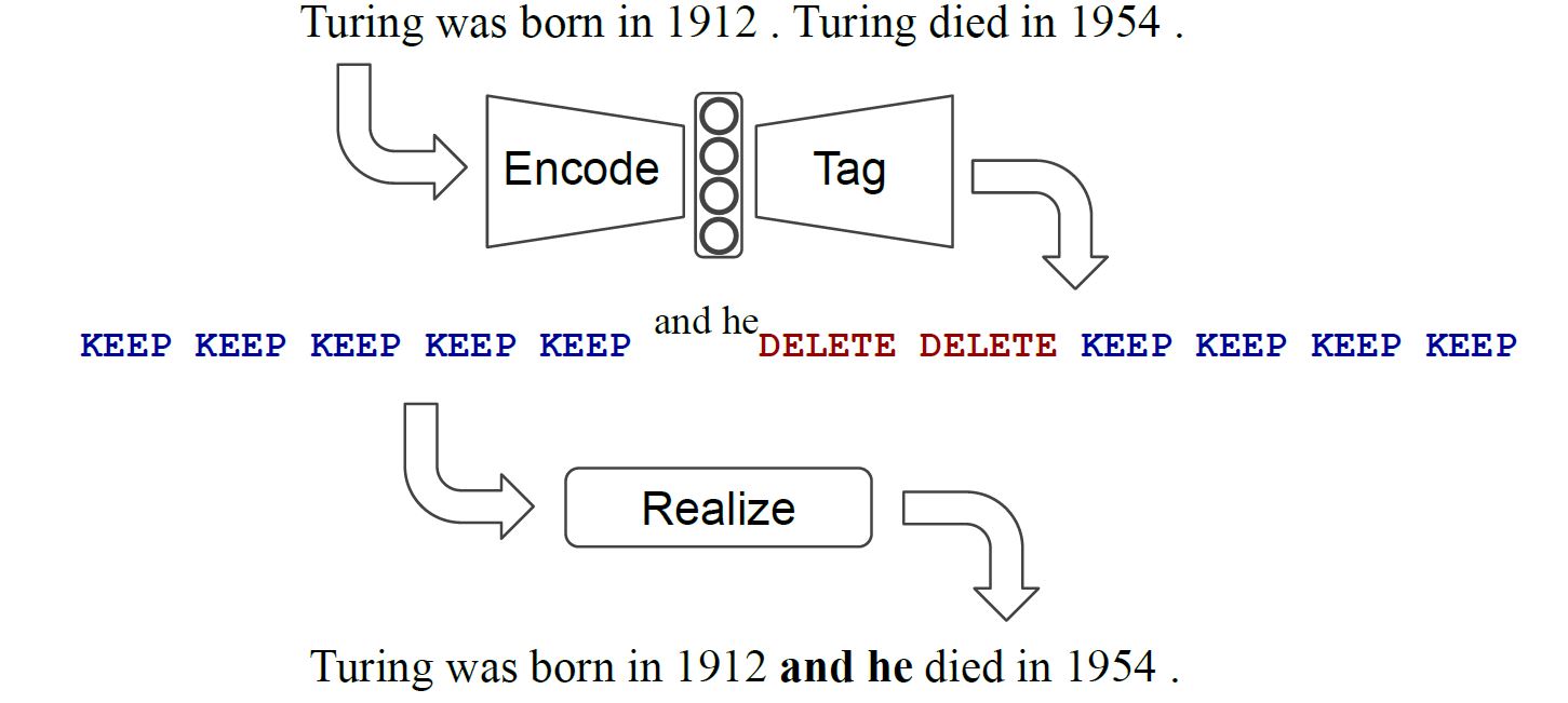
其实就是两个过程,一.将输入文本变编码成特殊标注,二.将标注解码成文本

四. 文本标注

4.1 Tag集构建(也就是label集构建)

一般情况,tag分为两个大类: base tag $B$和 add tag $P$。对于base tag,就是$KEEP$或者$DELETE$当前token;对于add tag,就是要添加一个词到token前面,添加的词来源于词表$V$。实际在工程中,将$B$和$P$结合来表示,即$^{P}B$,总的tag数量大约等于$B$的数量乘以$P$的数量,即$2|V|$。对于某些任务可以引入特定的tag,比如对于句子融合,可以引入$SWAP$,如下图。

4.1.1 词表V的构建

构建目标:

  1. 最小化词汇表规模;
  2. 最大化目标词语的比例

限制词汇表的词组数量可以减少相应输出的决策量;最大化目标词语的比例可以防止模型添加无效词。

构建过程:

通过$LCS$算法(longest common sequence,最长公共子序列,注意和最长公共子串不是一回事),找出输入和输出序列的最长公共子序列,输出剩下的序列,就是需要$add$的token,添加到词表$V$,词表中的词基于词频排序,然后选择$l$个常用的。

举个例子:soruce为“12345678”,target为”1264591”

​ 最长公共子序列为[‘1’, ‘2’, ‘4’, ‘5’]

​ 需要$add$的token为 [‘6’, ‘91’]

源码

1
2
3
4
5
6
7
8
9
10
11
12
13
14
15
16
17
18
19
20
21
22
23
24
25
26
27
28
29
30
31
32
33
34
35
36
37
38
39
40
41
42
43
44
45
46
47
48
49
50
51
52
53
54
55
56
57
58
59
60
61
62
63
64
65
66
67
def _lcs_table(source, target):
"""Returns the Longest Common Subsequence dynamic programming table."""
rows = len(source)
cols = len(target)
lcs_table = [[0] * (cols + 1) for _ in range(rows + 1)]
for i in range(1, rows + 1):
for j in range(1, cols + 1):
if source[i - 1] == target[j - 1]:
lcs_table[i][j] = lcs_table[i - 1][j - 1] + 1
else:
lcs_table[i][j] = max(lcs_table[i - 1][j], lcs_table[i][j - 1])
return lcs_table


def _backtrack(table, source, target, i, j):
"""Backtracks the Longest Common Subsequence table to reconstruct the LCS.

Args:
table: Precomputed LCS table.
source: List of source tokens.
target: List of target tokens.
i: Current row index.
j: Current column index.

Returns:
List of tokens corresponding to LCS.
"""
if i == 0 or j == 0:
return []
if source[i - 1] == target[j - 1]:
# Append the aligned token to output.
return _backtrack(table, source, target, i - 1, j - 1) + [target[j - 1]]
if table[i][j - 1] > table[i - 1][j]:
return _backtrack(table, source, target, i, j - 1)
else:
return _backtrack(table, source, target, i - 1, j)

def _compute_lcs(source, target):
# s1={1,3,4,5,6,7,7,8},s2={3,5,7,4,8,6,7,8,2} return 35778
table = _lcs_table(source, target)
return _backtrack(table, source, target, len(source), len(target))


def _get_added_phrases(source: Text, target: Text) -> Sequence[Text]:
"""
Computes the phrases that need to be added to the source to get the target.
"""
sep = ''
source_tokens = utils.get_token_list(source.lower())
target_tokens = utils.get_token_list(target.lower())
#compute Longest Common Subsequence
kept_tokens = _compute_lcs(source_tokens, target_tokens)
added_phrases = []
kept_idx = 0
phrase = []
for token in target_tokens:
if kept_idx < len(kept_tokens) and token == kept_tokens[kept_idx]:
kept_idx += 1
if phrase:
added_phrases.append(sep.join(phrase))
phrase = []
else:
phrase.append(token)
if phrase:
added_phrases.append(sep.join(phrase))
return added_phrases

词表位于文件label_map.txt.log,本人基于自己的数据集,内容如下所示

1
2
3
4
5
Idx Frequency  Coverage (%)   Phrase
1 19 94.22 址
2 15 95.27 单位
3 8 95.76 地
4 6 96.17 执勤

4.1.2 tag集

本人基于自己的数据集,得到的候选tag如下:

1
2
3
4
5
6
7
8
9
10
KEEP
DELETE
KEEP|址
DELETE|址
KEEP|单位
DELETE|单位
KEEP|地
DELETE|地
KEEP|执勤
DELETE|执勤

4.2 Converting Training Targets into Tags

paper上的伪代码:

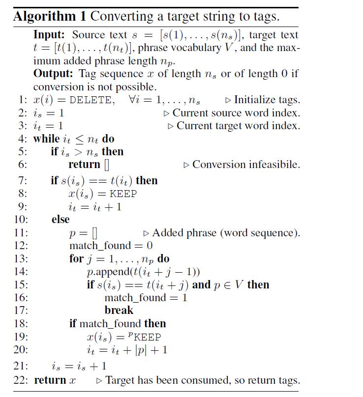
采用贪心策略,核心思想就是遍历$t$,先和$s$匹配,匹配上就$keep$,然后$i_t+j$,得到潜在的$add \ phrase \ p=t(i_t:i_t+j-1) $,然后判断$t(i_t+j)==s(i_s)\ and \ p\in V $

源码

和伪代码有一点不同,差异在于#####之间。

1
2
3
4
5
6
7
8
9
10
11
12
13
14
15
16
17
18
19
20
21
22
23
24
25
26
27
28
29
30
31
32
33
34
35
36
37
38
39
40
41
42
43
44
45
46
47
48
49
50
51
52
53
54
55
56
57
58
59
60
61
62
63
64
65
66
67
68
69
70
71
72
73
74
75
76
77
78
79
80
81
82
83
84
85
86
def _compute_single_tag(
self, source_token, target_token_idx,
target_tokens):
"""Computes a single tag.

The tag may match multiple target tokens (via tag.added_phrase) so we return
the next unmatched target token.

Args:
source_token: The token to be tagged.
target_token_idx: Index of the current target tag.
target_tokens: List of all target tokens.

Returns:
A tuple with (1) the computed tag and (2) the next target_token_idx.
"""
source_token = source_token.lower()
target_token = target_tokens[target_token_idx].lower()
if source_token == target_token:
return tagging.Tag('KEEP'), target_token_idx + 1
# source_token!=target_token
added_phrase = ''
for num_added_tokens in range(1, self._max_added_phrase_length + 1):
if target_token not in self._token_vocabulary:
break
added_phrase += (' ' if added_phrase else '') + target_token
next_target_token_idx = target_token_idx + num_added_tokens
if next_target_token_idx >= len(target_tokens):
break
target_token = target_tokens[next_target_token_idx].lower()
if (source_token == target_token and
added_phrase in self._phrase_vocabulary):
return tagging.Tag('KEEP|' + added_phrase), next_target_token_idx + 1
return tagging.Tag('DELETE'), target_token_idx


def _compute_tags_fixed_order(self, source_tokens, target_tokens):
"""Computes tags when the order of sources is fixed.

Args:
source_tokens: List of source tokens.
target_tokens: List of tokens to be obtained via edit operations.

Returns:
List of tagging.Tag objects. If the source couldn't be converted into the
target via tagging, returns an empty list.
"""
tags = [tagging.Tag('DELETE') for _ in source_tokens]
# Indices of the tokens currently being processed.
source_token_idx = 0
target_token_idx = 0
while target_token_idx < len(target_tokens):
tags[source_token_idx], target_token_idx = self._compute_single_tag(
source_tokens[source_token_idx], target_token_idx, target_tokens)
####################################################################################
# If we're adding a phrase and the previous source token(s) were deleted,
# we could add the phrase before a previously deleted token and still get
# the same realized output. For example:
# [DELETE, DELETE, KEEP|"what is"]
# and
# [DELETE|"what is", DELETE, KEEP]
# Would yield the same realized output. Experimentally, we noticed that
# the model works better / the learning task becomes easier when phrases
# are always added before the first deleted token. Also note that in the
# current implementation, this way of moving the added phrase backward is
# the only way a DELETE tag can have an added phrase, so sequences like
# [DELETE|"What", DELETE|"is"] will never be created.
if tags[source_token_idx].added_phrase:
# # the learning task becomes easier when phrases are always added before the first deleted token
first_deletion_idx = self._find_first_deletion_idx(
source_token_idx, tags)
if first_deletion_idx != source_token_idx:
tags[first_deletion_idx].added_phrase = (
tags[source_token_idx].added_phrase)
tags[source_token_idx].added_phrase = ''
########################################################################################
source_token_idx += 1
if source_token_idx >= len(tags):
break

# If all target tokens have been consumed, we have found a conversion and
# can return the tags. Note that if there are remaining source tokens, they
# are already marked deleted when initializing the tag list.
if target_token_idx >= len(target_tokens): # all target tokens have been consumed
return tags
return [] # TODO

缺陷

对于一些情况,无法还原,举个例子:

​ source:证件有效期截止日期 target:证件日期格式

​ 得不到tag结果

可以补充策略来修复bug

1
2
3
4
5
6
7
8
9
10
11
12
13
14
15
16
17
18
19
20
21
22
23
24
25
26
27
28
29
30
31
32
33
34
35
36
37
38
39
40
41
42
43
44
45
46
47
48
49
50
51
52
53
54
55
56
57
58
59
60
61
62
63
64
def _compute_tags_fixed_order(self, source_tokens, target_tokens):
"""Computes tags when the order of sources is fixed.

Args:
source_tokens: List of source tokens.
target_tokens: List of tokens to be obtained via edit operations.

Returns:
List of tagging.Tag objects. If the source couldn't be converted into the
target via tagging, returns an empty list.
"""


tags = [tagging.Tag('DELETE') for _ in source_tokens]
# Indices of the tokens currently being processed.
source_token_idx = 0
target_token_idx = 0
while target_token_idx < len(target_tokens):
tags[source_token_idx], target_token_idx = self._compute_single_tag(
source_tokens[source_token_idx], target_token_idx, target_tokens)
#########################################################################################
# If we're adding a phrase and the previous source token(s) were deleted,
# we could add the phrase before a previously deleted token and still get
# the same realized output. For example:
# [DELETE, DELETE, KEEP|"what is"]
# and
# [DELETE|"what is", DELETE, KEEP]
# Would yield the same realized output. Experimentally, we noticed that
# the model works better / the learning task becomes easier when phrases
# are always added before the first deleted token. Also note that in the
# current implementation, this way of moving the added phrase backward is
# the only way a DELETE tag can have an added phrase, so sequences like
# [DELETE|"What", DELETE|"is"] will never be created.
if tags[source_token_idx].added_phrase:
# # the learning task becomes easier when phrases are always added before the first deleted token
first_deletion_idx = self._find_first_deletion_idx(
source_token_idx, tags)
if first_deletion_idx != source_token_idx:
tags[first_deletion_idx].added_phrase = (
tags[source_token_idx].added_phrase)
tags[source_token_idx].added_phrase = ''
#######################################################################################

source_token_idx += 1
if source_token_idx >= len(tags):
break

# If all target tokens have been consumed, we have found a conversion and
# can return the tags. Note that if there are remaining source tokens, they
# are already marked deleted when initializing the tag list.
if target_token_idx >= len(target_tokens): # all target tokens have been consumed
return tags
####fix bug by lavine

###strategy1
added_phrase = "".join(target_tokens[target_token_idx:])
if added_phrase in self._phrase_vocabulary:
tags[-1] = tagging.Tag('DELETE|' + added_phrase)
print(''.join(source_tokens))
print(''.join(target_tokens))
print(str([str(tag) for tag in tags] if tags != None else None))
return tags
###strategy2
return [] # TODO

4.3 模型结构

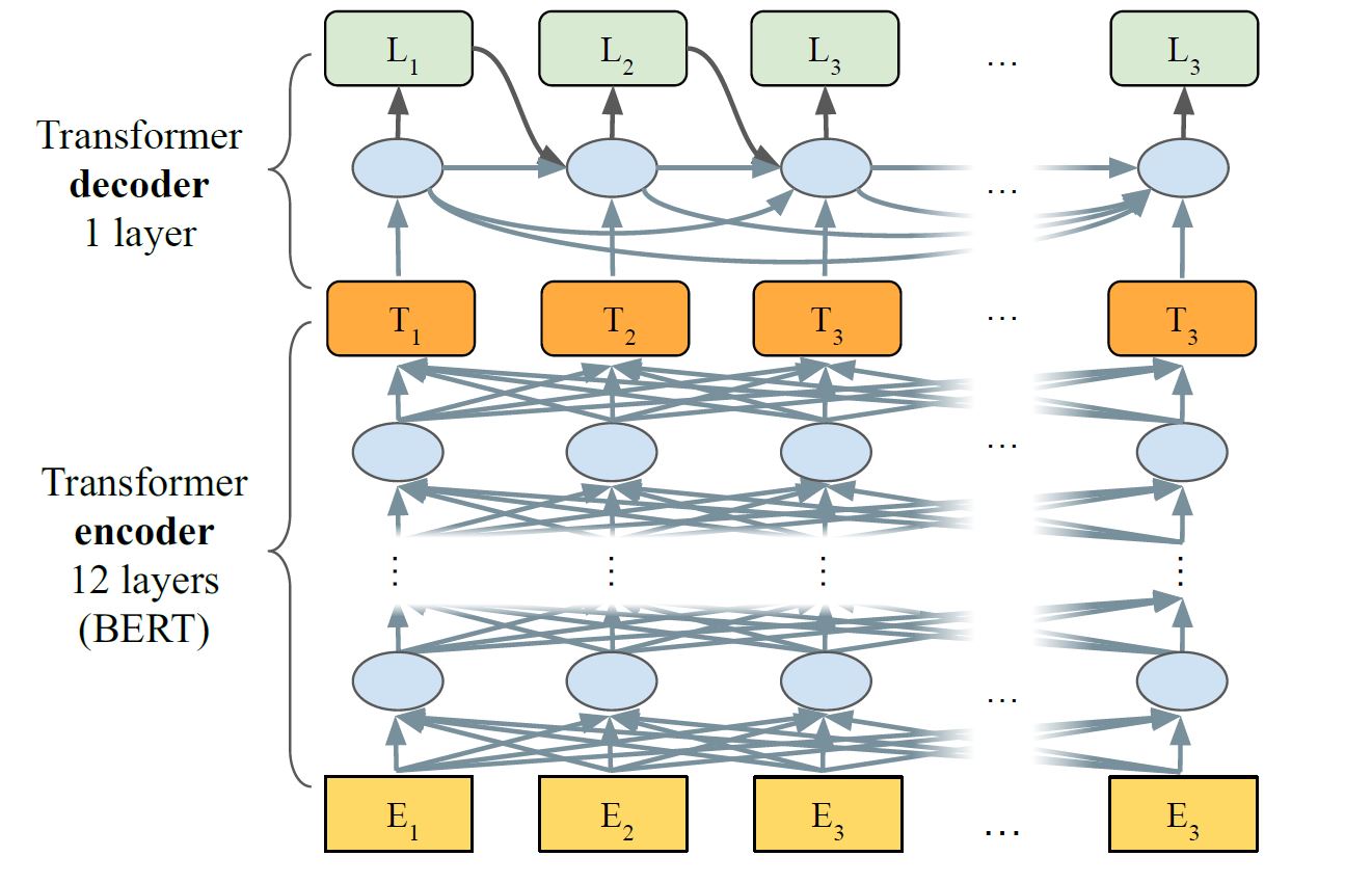
模型主要包含两个部分:1.encoder:generates activation vectors for each element in the input sequence 2.decoder:converts encoder activations into tag labels

4.3.1 encoder

由于$BERT$在sentence encoding tasks上做到state-of-the-art,所以使用$BERT$ 作为encoder部分。作者选择了$BERT_{base}$,包含12个self-attention层

4.3.2 decoder

在$BERT$原文中,对于标注任务采取了非常简单的decoder结构,即采用一层feed-forward作为decoder,把这种组合叫做$LASERTAGGER_{FF}$,这种结构的缺点在于预测的标注词相互独立,没有考虑标注词的关联性。

为了考虑标注词的关联性,decode使用了Transformer decoder,单向连接,记作$LASERTAGGER_{AR}$,这种encoder和decoder的组合的有点像BERT结合GPT的感觉decoder 和encoder在以下方面交流:(i) through a full attention over the sequence of encoder activations (ii) by directly consuming the encoder activation at the current step

4.4 loss

假设句子长度为n,tag数量为m, loss为n个m分类任务的和

五.realize

对于基本的tag,比如$KEEP$,$DELETE$,$ADD$,$realize$就是根据输入和tag直接转换就行;对于特殊的tag,需要一些特定操作,看情况维护规则。

六.评价指标

评价指标,不同任务不同评价指标

1 Sentence Fusion

Exact score :percentage of exactly correctly predicted fusions(类似accuracy)

SARI :average F1 scores of the added, kept, and deleted n-grams

2 Split and Rephrase

SARI

3 Abstractive Summarization

ROUGE-L

4 Grammatical Error Correction (GEC)

precision and recall, F0:5

七.实验结果

baseline: based on Transformer where both the encoder and decoder replicate the $BERT_{base}$ architecture

速度:1.$LASERTAGGER_{AR} $is already 10x faster than comparable-in-accuracy $SEQ2SEQ_{BERT}$ baseline. This difference is due to the former model using a 1-layer decoder (instead of 12 layers) and no encoder-decoder cross attention. 2.$LASERTAGGER_{FF}$ is more than 100x faster

其余结果参考paper

参考

https://arxiv.org/pdf/1909.01187.pdf
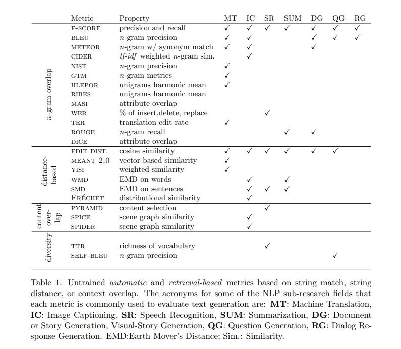
https://github.com/google-research/lasertagger

https://zhuanlan.zhihu.com/p/348109034

文本生成评价指标

1.BLEU

BLEU,全称为bilingual evaluation understudy,一般用于机器翻译和文本生成的评价,比较候选译文和参考译文里的重合程度,重合程度越高就认为译文质量越高,取值范围为[0,1]。

优点

  • 它的易于计算且速度快,特别是与人工翻译模型的输出对比;
  • 它应用范围广泛,这可以让你很轻松将模型与相同任务的基准作对比。

缺点

  • 它不考虑语义,句子结构
  • 不能很好地处理形态丰富的语句(BLEU原文建议大家配备4条翻译参考译文)
  • BLEU 指标偏向于较短的翻译结果(brevity penalty 没有想象中那么强)

1.1 完整式子

BLEU完整式子为:

1.2 $BP$

目的:$n-gram$匹配度可能会随着句子长度的变短而变好,比如,只翻译了一个词且对了,那么匹配度很高,为了避免这种评分的偏向性,引入长度惩罚因子

Brevity Penalty为长度惩罚因子,其中$l_c$表示机器翻译的译文长度,$l_s$表示参考答案的有效长度

1.3 $P_n$

人工译文表示为$s_j$,其中$j \in M$,$M$表示共有$M$个参考答案
翻译译文表示$c_i$,其中$i \in E$,$E$表示共有$E$个翻译
$n-gram$表示$n$个单词长度的词组集合,令$k$ 表示第$k$ 个词组,总共$K$个
$h_k(c_i)$表示第$k$个词组在翻译译文$c_i$出现的次数
$h_k(s_{j})$表示第$k$个词组在参考答案$s_{j}$出现的次数
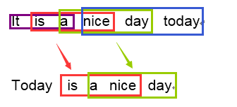
举例如下,例如:

    原文:今天天气不错

    机器译文:It is a nice day today

    人工译文:Today is a nice day

$1-gram$:

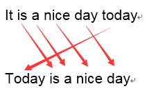
 可以看到机器译文一共6个词,有5个词语都命中的了参考译文,$P_1=\frac{5}{6}$

$3-gram$:

机器译文一共可以分为4个$3-gram$的词组,其中有2个可以命中参考译文,那么$P_3=\frac{2}{4}$

1.4 $W_n$

$W_n$表示$P_n$的权重,一般为加权平均,即$W_n=\frac{1}{N}$,其中$N$为$gram$的数量,一般不大于4
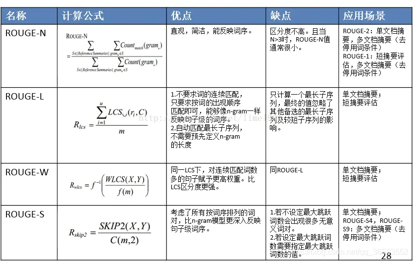
2 ROUGE

Recall-Oriented Understudy for Gisting Evaluation,可以看做是BLEU 的改进版,专注于召回率而非精度。换句话说,它会查看有多少个参考译句中的 n 元词组出现在了输出之中。

ROUGE大致分为四种(常用的是前两种): - ROUGE-N (将BLEU的精确率优化为召回率) - ROUGE-L (将BLEU的n-gram优化为公共子序列) - ROUGE-W (将ROUGE-L的连续匹配给予更高的奖励) - ROUGE-S (允许n-gram出现跳词(skip))

注意:

关于rouge包给出三个结果,而论文只有一个值,比如

1
[{'rouge-1': {'r': 1.0, 'p': 1.0, 'f': 0.999999995}, 'rouge-2': {'r': 0.0, 'p': 0.0, 'f': 0.0}, 'rouge-l': {'r': 1.0, 'p': 1.0, 'f': 0.999999995}}]

用“r”,recall就好了

3 NIST

4 METEOR

5 TER

参考文献

https://blog.csdn.net/qq_36533552/article/details/107444391

https://zhuanlan.zhihu.com/p/144182853

https://arxiv.org/pdf/2006.14799.pdf

https://www.cnblogs.com/by-dream/p/7679284.html

https://blog.csdn.net/qq_30232405/article/details/104219396

https://blog.csdn.net/u013521274/article/details/89460322

https://zhuanlan.zhihu.com/p/388720967

attention seq2seq

1.结构

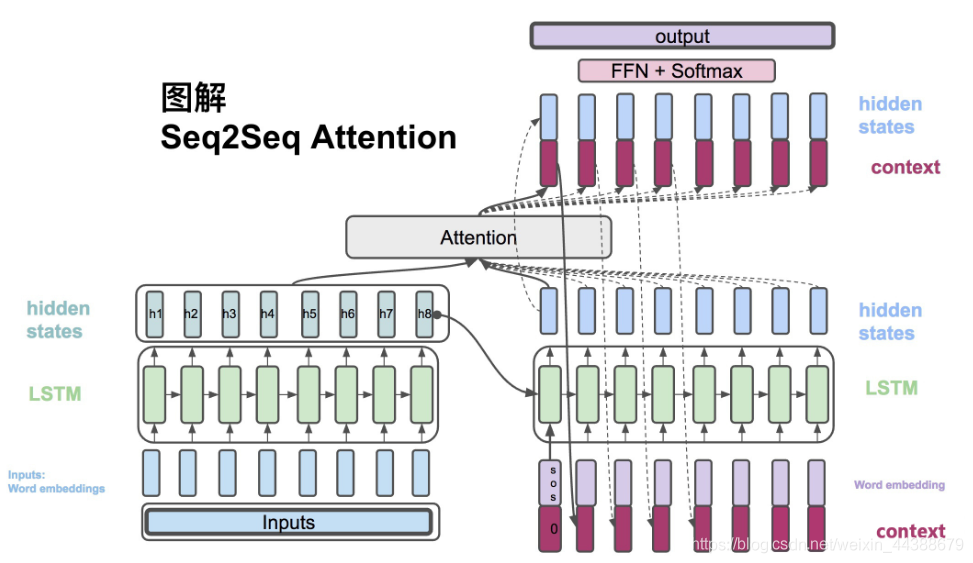
左边为encoder,对输入文本编码,右边为decoder,解码并应用。

整个流程的图解可以参考https://blog.csdn.net/weixin_44388679/article/details/102575223 中的“四、图解Attention Seq2Seq”,非常详细。

2.Teacher Forcing

在训练阶段,如果使用Teacher Forcing策略,那么目标句子单词的word embedding使用真值,否则使用预测结果;至于预测阶段不能使用Teacher Forcing。

beam search本质为介于蛮力与贪心之间的策略。对于贪心,每一级的输出只选择top1的结果作为下一级输入,然后top1的结果只是局部最优,不一定是全局最优,精度可能较低。对于蛮力,每级将全部结果输入下级,假设$L$为词表大小,那么最后一级的数据量为$L^{m}$,$m$为decoder 的cell数量,计算效率太低。对于beam search,每级选择top k作为下级输入,综合了效率和精度。

4 常见问题

0 为什么rnn based seq2seq不需要额外添加位置信息?

天然有位置信息(迭代顺序)

1 为什么rnn based seq2seq输入输出长度可变?

因为rnn based seq2seq是迭代进行的,所以长度可变

2 训练的时候要padding吗?

不用padding

参考

https://zhuanlan.zhihu.com/p/47929039

https://www.cnblogs.com/liuxiaochong/p/14399416.html

https://blog.csdn.net/thriving_fcl/article/details/74853556


:D 一言句子获取中...