ConSERT A Contrastive Framework for Self-Supervised Sentence Representation Transfer

https://arxiv.org/abs/2105.11741

https://tech.meituan.com/2021/06/03/acl-2021-consert-bert.html

1.背景

首先,BERT其自身导出的句向量(不经过Fine-tune,对所有词向量求平均)会出现“坍缩(Collapse)”现象,即所有的句子都倾向于编码到一个较小的空间区域内,如图。为了解决这个问题,将对比学习结合到finetune过程,借助无标签数据来提升模型的能力。

2.原理

给定一个类似BERT的预训练语言模型$\textbf{M}$,以及从目标领域数据分布中收集的无标签文本语料库$\mathcal{D}$,我们希望通过构建自监督任务在$\mathcal{D}$上对$\textbf{M}$进行Fine-tune,使得Fine-tune后的模型能够在目标任务(文本语义匹配)上表现最好。

2.1 整体框架

模型整体结构如上图所示,主要由三个部分组成

A data augmentation module that generates different views for input samples at the token embedding layer.

A shared BERT encoder that computes sentence representations for each input text. During training, we use the average pooling of the token embeddings at the last layer to obtain sentence representations.

A contrastive loss layer on top of the BERT encoder. It maximizes the agreement between one representation and its corresponding version that is augmented from the same sentence while keeping it distant from other sentence representations in the same batch.

对于任意一个句子输入$x$,得到其对应的两个增强向量$e_i=T_1(x),e_j=T_2(x),e_i,e_j\in \mathbb{R}^{L\times d}$,然后经过shared BERT encoder编码为$r_i,r_j$,其中$T_1,T_2$为不同的数据增强方式,$L$为句子$x$的长度,$d$为隐藏单元的数量。对于每个train step,从$\mathcal{D}$随机选取$N$个样本作为mini-batch,然后得到$2N$个增强样本,使用NT-Xent构造loss为

其中$sim(.)$为余弦相似度计算,$\tau$表示temperature,是一个超参数,实验中取0.1,$\mathbb{1}$是指示器,当$k=i$时,值为0。上式分子为正样本,分母为全部(但是基本为负样本,所以可以看成负样本),所以loss变小就是让分子变大,分母变小,也就是让正样本相似度变大,负样本相似度变小

2.2 数据增强策略

显式生成增强样本的方法包括:回译、同义词替换、意译等,然而这些方法一方面不一定能保证语义一致。所以考虑了在Embedding层隐式生成增强样本的方法。

  • 对抗攻击(Adversarial Attack):这一方法通过梯度反传生成对抗扰动,将该扰动加到原本的Embedding矩阵上,就能得到增强后的样本。由于生成对抗扰动需要梯度反传,因此这一数据增强方法仅适用于有监督训练的场景。

  • 打乱词序(Token Shuffling):这一方法扰乱输入样本的词序。由于Transformer结构没有“位置”的概念,模型对Token位置的感知全靠Embedding中的Position Ids得到。因此在实现上,我们只需要将Position Ids进行Shuffle即可。

  • 裁剪(Cutoff)

    :又可以进一步分为两种:

    • Token Cutoff:随机选取Token,将对应Token的Embedding整行置为零。
    • Feature Cutoff:随机选取Embedding的Feature,将选取的Feature维度整列置为零。
  • Dropout:Embedding中的每一个元素都以一定概率置为零,与Cutoff不同的是,该方法并没有按行或者按列的约束。

2.3 融合监督信号

除了无监督训练以外,作者给出3种进一步融合监督信号的策略,以NLI任务为例:

Joint training (joint):

Supervised training then unsupervised transfer (sup-unsup):

first train the model with $\mathcal{L}_{ce}$on NLI dataset, then use $\mathcal{L}_{con}$to finetune it on the target dataset.

Joint training then unsupervised transfer (joint-unsup):

first train the model with the $\mathcal{L}_{joint}$on NLI dataset, then use $\mathcal{L}_{con }$to fine-tune it on the target dataset.

3.定性分析

后又发现BERT句向量表示的坍缩和句子中的高频词有关。具体来说,当通过平均词向量的方式计算句向量时,那些高频词的词向量将会主导句向量,使之难以体现其原本的语义。当计算句向量时去除若干高频词时,坍缩现象可以在一定程度上得到缓解(如图2蓝色曲线所示)。

4 实验结果

4.1 Unsupervised Results

4.2 Supervised Results

gpt

GPT三部曲宣告NLP的“预训练+微调”时代的崛起和走向辉煌。

原文分别为:

《Improving Language Understanding by Generative Pre-Training》

《Language Models are Unsupervised Multitask Learners》

《Language Models are Few-Shot Learners》

1.GPT1

img

模型的整体结构如上图所示。使用过程过程分为两步:第一步预训练,利用大量语料学习得到high-capacity的语言模型;第二步是fine_tuning,利用标签数据使其拟合到特定任务。

1.1 Unsupervised pre-training

作者将transformer decoder中Encoder-Decoder Attention层去掉后作为基本单元,然后多层堆叠作为语言模型的主体,然后将输出经过一个softmax层,来得到目标词的输出分布:

其中$U=\{u_{-k},…,u_{-1}\}$ 是预测词$u $前$k$个token的独热编码序列,$n$是模型的层数,$W_e$是token embedding matrix,$W_p$是position embedding matrix。

给定一个无监督的语料库$\mathcal{U}$,use a standard language modeling objective to maximize the following likelihood

其中$k$ 是上下文窗口大小。

1.2 Supervised fine-tuning

对于数据集$\mathcal{C}$,有数据$(x^1,x^2,…,x^m,y)$

其中$W_y$为全连接层的参数

作者发现,使用语言模型来辅助监督学习进行微调,有两个好处:

  1. 提高监督模型的泛化能力;
  2. 加速收敛。

所以,最终下游使用的监督模型损失函数为:

1.3 Task-specific input transformations

所有的输入文本都会加上开始和结合token$(s),(e)$

分类

分类过程可如上1.2,输入表示为$[(s);Context;(e)]$

文本蕴含

将输入拼接成$[(s); premise; ($) ; hypothesis ; (e)]$

相似度

由于文本相似度与两个比较文本的前后顺序没有关系,因此将两种文本顺序都考虑进来,如上图所示

问答与常识推理

假设文档为$z$,问题为$q$,一系列答案为$\{a_k\}$,将其输入表示为$[(s); z; q; ($); a_k;(e)]$,然后多个回答组合的形式,如上图。

2.GPT2

总结就是:多任务预训练+超大数据集+超大规模模型。通过一个超大数据集涵盖NLP的大多任务,然后使用一个超大规模模型进行多任务预训练,使其无需任何下游任务的finetune就可以做到多个NLP任务的SOTA。举个例子,拿高考为例,人的智力和脑容量可以理解为参数大小,由于个体差异,可以将不同的学生理解为不同参数量的模型,卷子可以理解为数据集,不同的学科可以理解为不同任务。GPT2有点类似学霸,就是有超高的智力和脑容量,然后刷大量不同学科的题目,因此对高考这个多任务的下游任务就可以取得好成绩。

GPT2相对于GPT1有哪些不同呢?

  1. GPT2去掉了fine-tuning:不再针对不同任务分别进行微调建模,模型会自动识别出来需要做什么任务。这就好比一个人博览群书,你问他什么类型的问题,他都可以顺手拈来,GPT2就是这样一个博览群书的模型。

  2. 超大数据集:WebText,该数据集做了一些简单的数据清理,并且实验结果表明目前模型仍然处于一个欠拟合的情况。

  3. 增加网络参数:GPT2将Transformer堆叠的层数增加到48层,隐层的维度为1600,参数量更是达到了15亿。15亿什么概念呢,Bert的参数量也才只有3亿哦~当然,这样的参数量也不是说谁都能达到的,这也得取决于money的多少啊~

  4. 调整transformer:将layer normalization放到每个sub-block之前,并在最后一个transformer后再增加一个layer normalization,如下图。

  5. 输入表示:GPT2采用了BPE这种subword的结构作为输入

  6. 其他:GPT2将词汇表数量增加到50257个;最大的上下文大小 (context size) 从GPT的512提升到了1024 tokens;batchsize增加到512。

GPT2的输入是完全的文本,什么提示都不加吗?

当然不是,它也会加入提示词,比如:$TL;DR:$,GPT2模型就会知道是做摘要工作了,输入的格式就是 $文本+TL;DR:$,然后就等待输出就行了~

3.GPT3

GPT3,这是一种具有1750亿个参数的超大规模模型,比GPT2大100倍,感觉真是进入算力时代了。距离个人用户太远了,就不深挖了。

参考

https://zhuanlan.zhihu.com/p/146719974

https://zhuanlan.zhihu.com/p/125139937

https://www.cnblogs.com/yifanrensheng/p/13167796.html#_label1_0

https://www.jianshu.com/p/96c5d5d5c468

https://blog.csdn.net/qq_35128926/article/details/111399679

https://zhuanlan.zhihu.com/p/96791725

https://terrifyzhao.github.io/2019/02/18/GPT2.0%E8%AE%BA%E6%96%87%E8%A7%A3%E8%AF%BB.html

https://zhuanlan.zhihu.com/p/56865533

 NLP PTM
  
 PTM

TextCNN TextRNN TextRCNN

1.TextCNN (Convolutional Neural Networks for Sentence Classification)

原文 https://arxiv.org/abs/1408.5882

调参论文 https://arxiv.org/abs/1510.03820

模型的整体结构如上所示。Feature Map是输入图像经过神经网络卷积产生的结果,filter是卷积核。

输入表示:

假设输入文本的长度为$n$,对于长度不够的需要做padding,任意一个单词可以用一个$k$维的向量表示,即$X_i \in \mathbb{R}^{k}$,那么一个句子可以表示为

其中$\oplus$是向量拼接操作,$X_{1:n} \in \mathbb{R}^{nk\times 1}$。

卷积

对于某个滑窗$X_{i,i+h-1}=\{X_i,X_{i+1},…,X_{i+h-1}\}$经过某个卷积核$W_j$可得

其中$f=tanh(\cdot)$,$W_j\in \mathbb{R}^{ 1\times hk},c_{i,j} $是标量

假设卷积通道数为$m$,在NLP中,卷积滑动步伐$k=1$,那么经过卷积层后得到的完整的特征矩阵为

其中$C \in \mathbb{R}^{(n-h+1)\times m}$

maxpooling

全连接

然后将$\hat{C}$接个全连接,就可以做分类或者回归任务了。

2.TextRNN (Recurrent Neural Network for Text Classification with Multi-Task Learning)

原文 https://www.ijcai.org/Proceedings/16/Papers/408.pdf

该文的场景为Recurrent Neural Network for Text Classification with Multi-Task Learning,就是论文的题目。文中给出了三种结构,如上图所示,图中的RNN单元为LSTM。

Model-I: Uniform-Layer Architecture

对于任务$m$,输入$\hat X_t$包含两个部分

其中$X_{t}^{(m)}$表示特定任务的词向量,$X_{t}^{(s)}$表示共享的词向量,$\oplus$表示向量拼接的操作。

Model-II: Coupled-Layer Architecture

Model-III: Shared-Layer Architecture

3.TextRCNN(Recurrent Convolutional Neural Networks for Text Classification)

原文 https://www.deeplearningitalia.com/wp-content/uploads/2018/03/Recurrent-Convolutional-Neural-Networks-for-Text-Classification.pdf

整体结构如上图所示,解释一下为啥叫RCNN,一般的 CNN 网络,都是卷积层 + 池化层,这里是将卷积层换成了双向 RNN,所以结果是,双向 RNN + 池化层。作者原话为:From the perspective of convolutional neural networks, the recurrent structure we previously mentioned is the convolutional layer.

词语表示

对于一个词语$w_i$,可以用一个三元组表示为

其中$e(w_i)$表示$w_i$的词向量,$c_l(w_i)$表示$w_i$句子左边的内容的向量表示,$c_r(w_i)$表示$w_i$句子右边的内容的向量表示,用式子表示如下

然后将$x_i$经过全连接得到$y_i^{(2)}$,$y_i^{(2)}$is a latent semantic vector

语句表示

获取众多的词语表示后,通过max-pooling得到句子表示

然后接全连接和softmax

参考

https://www.cnblogs.com/wangduo/p/6773601.html

ELMo(Deep contextualized word representations)

引入了新的深度考虑上下文的词语表示,模型考虑了两个方面:(1)词语的复杂特性,包括语法和语义,(2)在语境中的不同含义。模型使用了深度双向语言模型,并且在大预料库上做了预训练。这个模型可以很方便地和现有的模型结合,并且在NLP的6个任务上取得了SOTA。作者还揭露了预训练网络的深层构件是关键,这使得下游模型能够混合不同类型的半监督信号。

3 ELMo: Embeddings from Language Models

模型的整体机构如上所示,由左右两个单向的多层LSTM网络构成,左边为正向,右边为反向。

3.1 Bidirectional language models(预训练)

假定一个句子有$N$个token,分别为$(t_1,t_2,…,t_N)$,正向的语言模型的句子概率为:

反向的语言模型的句子概率为:

得到正向和反向的语言后,将其结合可以得到双向的语言模型,这里取对数表示为:

其中$\Theta_x$为token表示的参数,$\Theta_s$为softmax层的参数,$\overrightarrow{\Theta}_{LSTM}$表示前向语言模型的参数,$\overleftarrow{\Theta}_{LSTM}$表示反向语言模型的参数。

3.2 ELMo(如何表示词向量)

得到$L$层的预训练双向深度语言模型后,对于token $t_k$,一共包含了$2L+1$个相关的表示,集合如下

注意$h_{k,0}^{LM}=x_{k}^{LM},h_{k,j}^{LM}=[\overrightarrow{h^{LM}_{k,j}};\overleftarrow{h^{LM}_{k,j}}]$,其中$x_{k}^{LM}$为token表示,$\overrightarrow{h^{LM}_{k,j}},\overleftarrow{h^{LM}_{k,j}}$分别为正反向语言模型的表示

对于下游任务,需要将$2L+1$个表示压缩到一个向量$ELmo_k^{task}$,最简单的做法是只取顶层的表示,即

更加通用的做法为线形组合输出,如下图,公式表达为

其中$\gamma^{task}$用于缩放向量,$s_{j}^{task}$表示权重,通过下游任务学习。

3.3 Using biLMs for supervised NLP tasks(fine tune)

对于下游任务模型,可以得到不考虑上下文的静态词向量$x_k$和考虑上下文的向量表示$h_k$

对于一部分任务,将$x_k$和$ ELMo_k^{task}$ 拼接作为下游任务的特征:$[x_k;ELMo_k^{task}]$

对于一部分任务,将 $h_k$和 $ ELMo_k^{task}$ 拼接可提升效果:$[h_k;ELMo_k^{task}]$

参考

https://blog.csdn.net/linchuhai/article/details/97170541

https://zhuanlan.zhihu.com/p/63115885

https://zhuanlan.zhihu.com/p/88993965

https://arxiv.org/abs/1802.05365

 NLP PTM
  

Pre-trained Models for Natural Language Processing A Survey

原文内容很丰富,慢慢学习更新。

摘要

这篇综述从language representation learning入手,然后全面的阐述Pre-trained Models的原理,结构以及downstream任务,最后还罗列了PTM的未来发展方向。该综述目的旨在为NLP小白,PTM小白做引路人,感人。

1.Introduction

随着深度学习的发展,许多深度学习技术被应用在NLP,比如CNN,RNN,GNN以及attention。

尽管NLP任务的取得很大成功,但是和CV比较,性能提高可能不是非常明显。这主要是因为NLP任务的数据集都非常小(除了机器翻译),然而深度网络参数非常多,没有足够的数据支撑网络训练会导致过拟合问题。

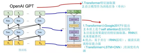
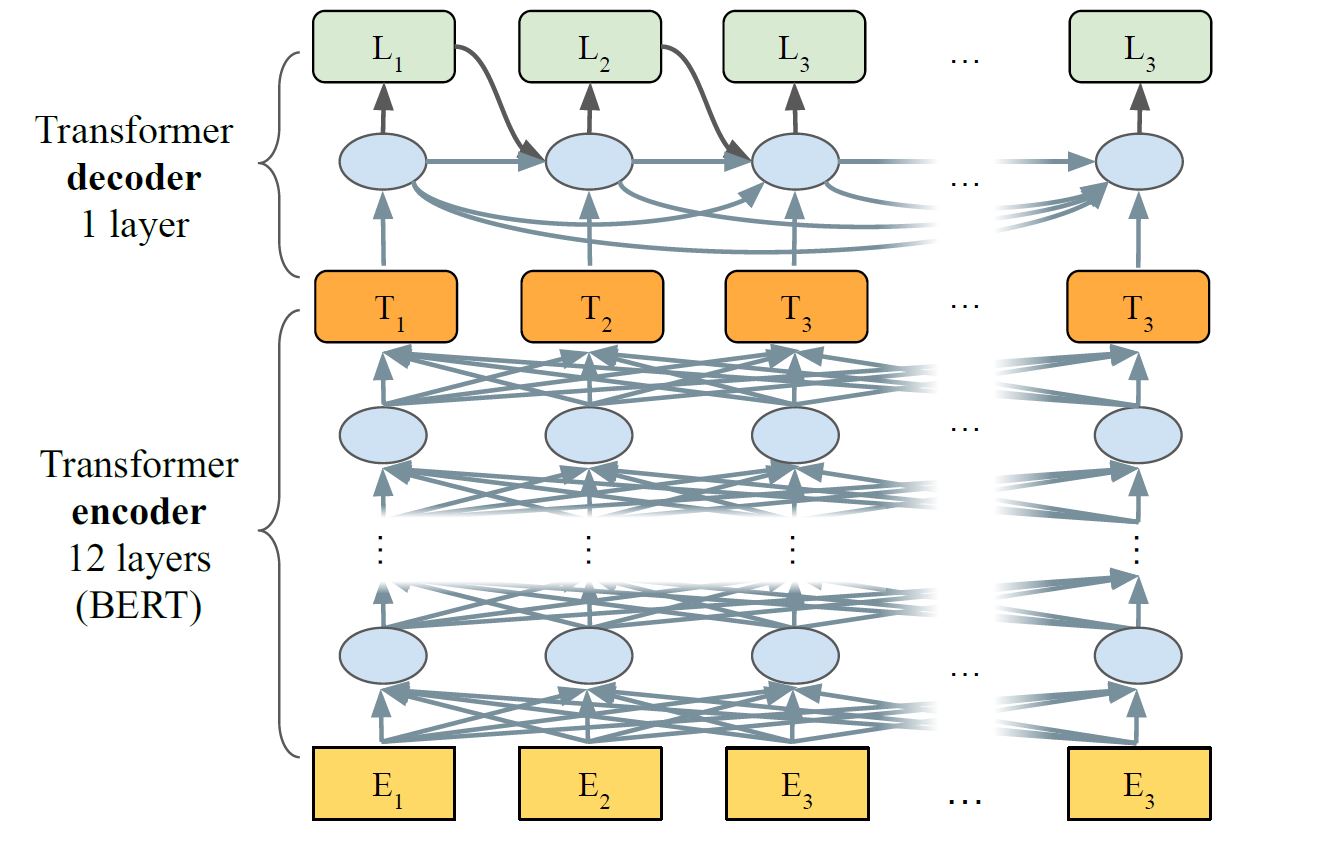
最近,大量工作表明,预先训练的模型(PTMs),在大型语料库上可以学习通用语言表示,这有利于下游NLP任务可以避免从零开始训练新模型。随着算力的发展,深度模型(例如,transformer)的出现和训练技巧的不断调高,PTM的结构从浅层发展成深层。第一代PTM被用于Non-contextual word Embedding。由于下游任务不需要这些模型本身,只需要训练好的词向量矩阵,因此对于现在的算力,这些模型非常浅层,比如Skip-Gram和GloVe。虽然这些预训练词向量可以捕获词语的语义,但它们不受上下文限制,无法捕获上下文中的高级含义,某些任务会失效,例如多义词,句法结构,语义角色、回指。第二代PTM关注Contextual word embeddings,比如BERT,GPT等。这些编码器任然需要通过下游任务在上下文中表示词语。

2.Background

2.1 Language Representation Learning

The core idea of distributed representation is to describe the meaning of a piece of text by low-dimensional real-valued vectors. And each dimension of the vector has no corresponding sense, while the whole represents a concrete concept.

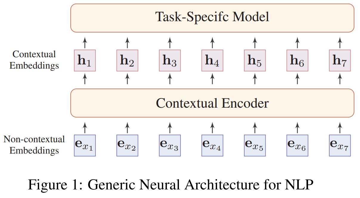
Non-contextual Embeddings

这一步主要是将分割的字符,比如图中的$x$,变成向量表达$e_x \in \mathbb{R}^{D_e}$,$D_e$是词向量维度。向量化过程就是基于一个离线训练的词向量矩阵$E\in \mathbb{R}^{D_e\times |\mathcal{V}|} $做查找,$\mathcal{V}$是词汇表。

这个过程主要有两个问题。第一个是这个词向量是静态的,没有考虑上下文含义,无法处理多义词。第二个是oov问题,许多算法可以缓解这个问题,比如基于character level,比如基于subword,subword算法有BPE,CharCNN等。

Contextual Embeddings

To address the issue of polysemous and the context-dependent nature of words, we need distinguish the semantics of words in different contexts:

其中$f_{enc}(\cdot)$为深度编码器。$\textbf{h}_t$就是contextual embedding或者dynamical embedding。

2.2 Neural Contextual Encoders

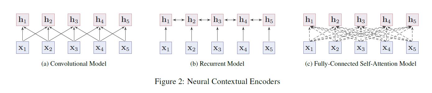
可以分成两类,sequence models and non-sequence models。

2.2.1 sequence models

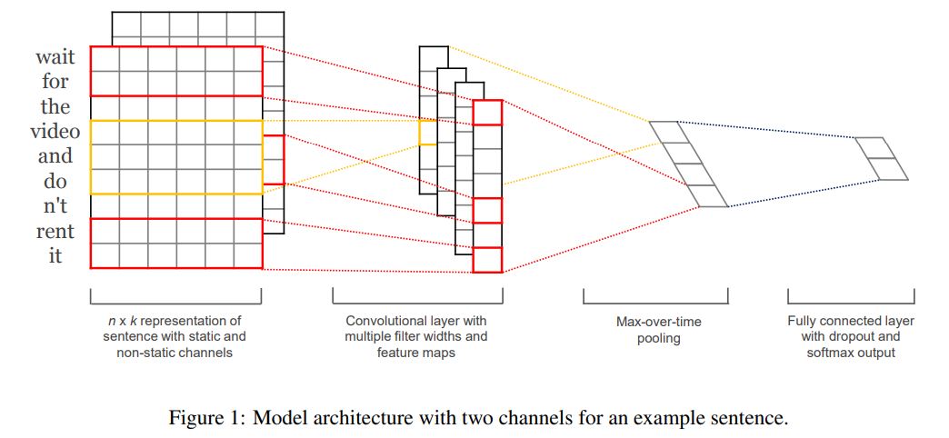
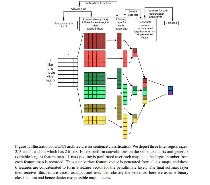
sequence models 分为两类,Convolutional Models和Recurrent Models,见上图。
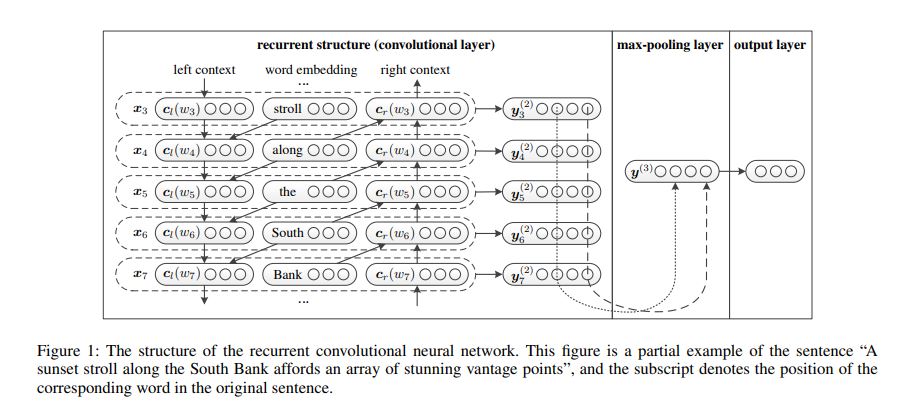
Convolutional

Convolutional models take the embeddings of words in the input sentence and capture the meaning of a word by aggregating the local information from its neighbors by convolution operations
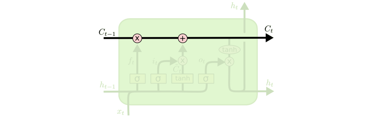
Recurrent

Recurrent models capture the contextual representations of words with short memory, such as LSTMs and GRUs . In practice, bi-directional LSTMs or GRUs are used to collect information from both sides of a word, but its performance is often affected by the long-term dependency problem.

2.2.2 non-sequence models

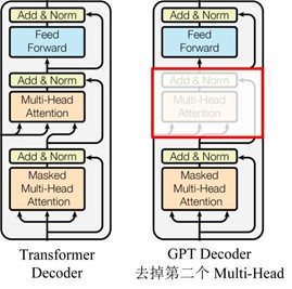
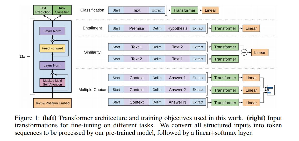
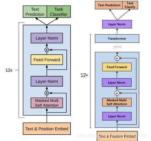
transformer: model the relation of every two words

2.2.3 Analysis

Sequence models:

1.Sequence models learn the contextual representation of the word with locality bias and are hard to capture the long-range interactions between words.

2.Nevertheless, sequence models are usually easy to train and get good results for various NLP tasks.

fully-connected self-attention model:

1.can directly model the dependency between every two words in a sequence, which is more powerful and suitable to model long range dependency of language

2.However, due to its heavy structure and less model bias, the Transformer usually requires a large training corpus and is easy to overfit on small or modestly-sized datasets

结论:the Transformer has become the mainstream architecture of PTMs due to its powerful capacity.

2.3 Why Pre-training?

  1. Pre-training on the huge text corpus can learn universal language representations and help with the downstream tasks.
  2. Pre-training provides a better model initialization,which usually leads to a better generalization performance and speeds up convergence on the target task.
  3. Pre-training can be regarded as a kind of regularization to avoid overfitting on small data

3 Overview of PTMs

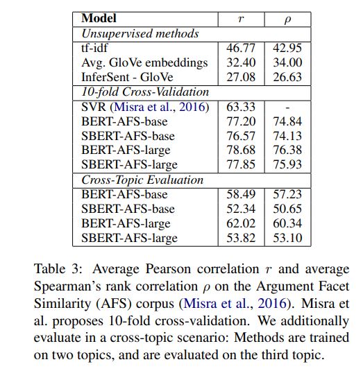
3.1 Pre-training Tasks

预训练任务对于学习通用语言表示至关重要。通常,这些预训练任务应具有挑战性,并拥有大量训练数据。在本节中,我们将预训练任务分成三个类别:Supervised learning、Unsupervised learning和Self-Supervised learning。

Self-Supervised learning: is a blend of supervised learning and unsupervised learning. The learning paradigm of SSL is entirely the same as supervised learning, but the labels of training data are generated automatically. The key idea of SSL is to predict any part of the input from other parts in some form. For example, the masked language model (MLM) is a self-supervised task that attempts to predict the masked words in a sentence given the rest words.

接下来基于介绍常用的基于Self-Supervised learning的预训练任务。

3.1.1 Language Modeling (LM)

3.1.2 Masked Language Modeling (MLM)

3.1.3 Permuted Language Modeling (PLM)

3.1.4 Denoising Autoencoder (DAE)

3.1.5 Contrastive Learning (CTL)

nsp也属于CTL

https://zhuanlan.zhihu.com/p/360892229

3.1.6 Others

3.2 Taxonomy of PTMs

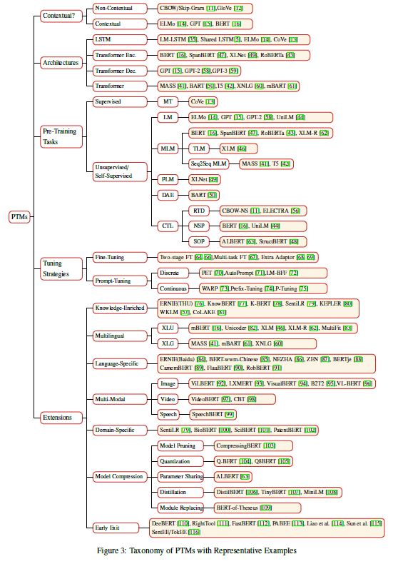
作者从以下四个角度,即Representation Type,Architectures,Pre-Training Task Types,Extensions,对现有的PTM分类,分类结果如上。图和这里有一点不统一,是作者没注意?图里有5个类别,多了Tuning Strategies,而且Representation Type在图中为Contextual?。

3.3 Model Analysis

4 Extensions of PTMs

4.1 Knowledge-Enriched PTMs

4.2 Multilingual and Language-Specific PTMs

4.3 Multi-Modal PTMs

4.4 Domain-Specific and Task-Specific PTMs

4.5 Model Compression

5 Adapting PTMs to Downstream Tasks

虽然PTM学习了很多通用知识,但是如何将这些知识有效应用到下游任务是个挑战。

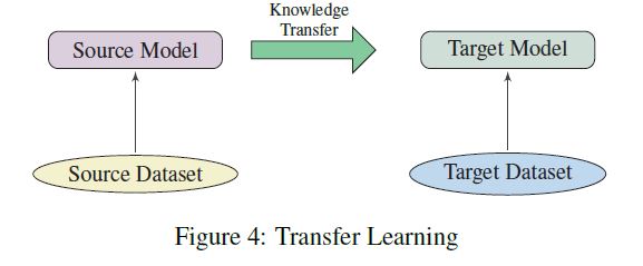
5.1 Transfer Learning

Transfer learning is to adapt the knowledge from a source task (or domain) to a target task (or domain).如下图。

5.2 How to Transfer?

5.2.1 Choosing appropriate pre-training task, model architecture and corpus

5.2.2 Choosing appropriate layers

使用哪些层参与下游任务

选择的层model1+下游任务model2

对于深度模型的不同层,捕获的知识是不同的,比如说词性标注,句法分析,长期依赖,语义角色,协同引用。对于RNN based的模型,研究表明多层的LSTM编码器的不同层对于不同任务的表现不一样。对于transformer based 的模型,基本的句法理解在网络的浅层出现,然而高级的语义理解在深层出现。

用$\textbf{H}^{l}(1<=l<=L)$表示PTM的第$l$层的representation,$g(\cdot)$为特定的任务模型。有以下几种方法选择representation:
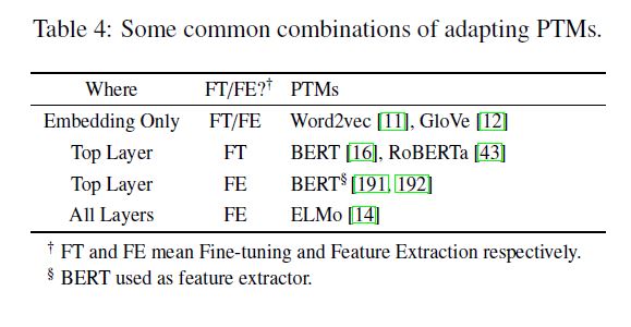
a) Embedding Only

choose only the pre-trained static embeddings,即$g(\textbf{H}^{1})$

b) Top Layer

选择顶层的representation,然后接入特定的任务模型,即$g(\textbf{H}^{L})$

c) All Layers

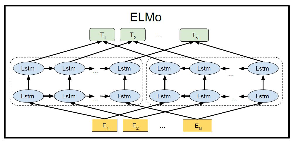
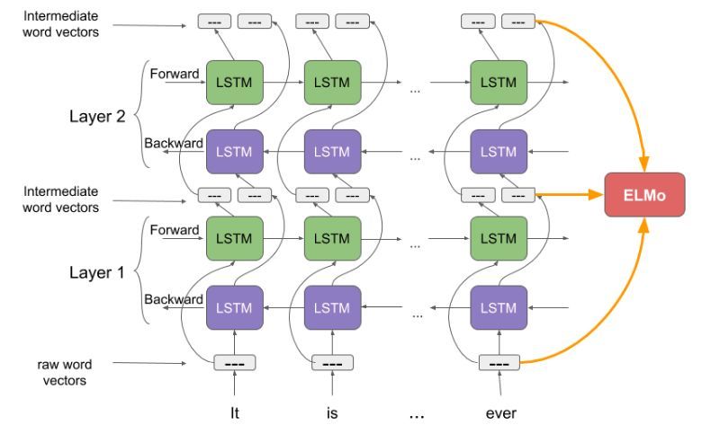
输入全部层的representation,让模型自动选择最合适的层次,然后接入特定的任务模型,比如ELMo,式子如下

其中$\alpha$ is the softmax-normalized weight for layer $l$ and $\gamma$ is a scalar to scale the vectors output by pre-trained model

5.2.3 To tune or not to tune?

总共有两种常用的模型迁移方式:feature extraction (where the pre-trained parameters are frozen), and fine-tuning (where the pre-trained parameters are unfrozen and fine-tuned).

选择的层model1参数是否固定,model2一定要训练

bert 只有top layer finetune????

5.3 Fine-Tuning Strategies

Two-stage fine-tuning

第一阶段为中间任务,第二阶段为目标任务

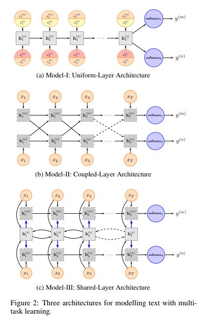
Multi-task fine-tuning

multi-task learning and pre-training are complementary technologies.

Fine-tuning with extra adaptation modules

The main drawback of fine-tuning is its parameter ineffciency: every downstream task has its own fine-tuned parameters. Therefore, a better solution is to inject some fine-tunable adaptation modules into PTMs while the original parameters are fixed.

Others

self-ensemble ,self-distillation,gradual unfreezing,sequential unfreezing

参考

https://arxiv.org/pdf/2003.08271v4.pdf

 NLP PTM
  
 PTM

word2vec

一.原理

两种训练模型

  • 如果是用一个词语作为输入,来预测它周围的上下文,那这个模型叫做『Skip-gram 模型』
  • 而如果是拿一个词语的上下文作为输入,来预测这个词语本身,则是 『CBOW 模型』

训练技巧

hierarchical softmax 和 negative sampling

二.代码

训练代码

1
2
3
4
5
6
7
8
9
10
11
12
13
from gensim.models.word2vec import Word2Vec
import pandas as pd
from gensim import models
import jieba


###train
data=pd.read_csv(data_path)
sentences=data.tolist()
model= Word2Vec()
model.build_vocab(sentences)
model.train(sentences,total_examples = model.corpus_count,epochs = 5)
model.save(model_path)

词向量矩阵

1
2
3
4
5
6
7
8
from gensim import models
if __name__ == '__main__':
model=models.KeyedVectors.load_word2vec_format(model_path,binary=True)
print(model.vectors) ##(779845, 400))
print("\n")
print(model.index_to_key)
print("\n")
print(model["的"])
1
2
3
4
5
array([[-1.3980628e+00, -4.6281612e-01,  5.8368486e-01, ...,         5.3952241e-01,  4.4697687e-01,  1.3505782e+00],       [ 4.9143720e-01, -1.4818899e-01, -2.8366420e-01, ...,         1.1110669e+00,  2.1992767e-01,  7.0457202e-01],       [-8.5650706e-01,  8.2832746e-02, -8.4218192e-01, ...,         2.1654253e+00,  6.4846051e-01, -5.7714492e-01],       ...,       [ 7.5072781e-03, -1.3543828e-02,  2.3101490e-02, ...,         4.2363801e-03, -5.6749382e-03,  6.3404259e-03],       [-2.6244391e-04, -3.0459568e-02,  5.9752418e-03, ...,         1.7844304e-02, -4.7109672e-04,  7.7916058e-03],       [ 7.2062697e-04, -6.5988898e-03,  1.1346856e-02, ...,        -3.7340564e-03, -1.8825980e-02,  2.7245486e-03]], dtype=float32)

[',', '的', '。', '、', '0', '1', '在', '”', '2', '了', '“', '和', '是', '5', ...]

array([ 4.9143720e-01, -1.4818899e-01, -2.8366420e-01, -3.6405793e-01, 1.0851435e-01, 4.9507666e-02, -7.1219063e-01, -5.4614645e-01, -1.3581418e+00, 3.0274218e-01, 6.1700332e-01, 3.5553512e-01, 1.6602433e+00, 7.5298291e-01, -1.4151905e-01, -2.1077128e-01, -2.6325354e-01, 1.6108564e+00, -4.6750236e-01, -1.6261842e+00, 1.3063166e-01, 8.0702168e-01, 4.0011466e-01, 1.2198541e+00, -6.2879241e-01, ... 2.1928079e-01, 7.1725255e-01, -2.3430648e-01, -1.2066336e+00, 9.7590965e-01, -1.5906478e-01, -3.5802779e-01, -3.8005975e-01, 1.9056025e-01, 1.1110669e+00, 2.1992767e-01, 7.0457202e-01], dtype=float32)

参考

https://zhuanlan.zhihu.com/p/26306795

https://arxiv.org/abs/1301.3781v3

https://arxiv.org/abs/1405.4053

Neural Graph Matching Networks for Chinese Short Text Matching

https://aclanthology.org/2020.acl-main.547.pdf

1.摘要

对于中文短文本匹配,通常基于词粒度而不是字粒度。但是分词结果可能是错误的、模糊的或不一致的,从而损害最终的匹配性能。比如下图:字符序列“南京市长江大桥”经过不同的分词可能表达为不同的意思。

为了解决这个问题,作者提出了一种基于图神经网络的中文短文本匹配方法。不是将句子分割成一个单词序列,而是保留所有可能的分割路径,形成一个Lattice(segment1,segment2,segment3),如上图所示。

2.问题定义

将两个待匹配中文短文本分别定义为$S_a=\left \{ C_1^a,C_2^a,…,C_{t_a}^a \right \}$,$S_b=\left \{ C_1^b,C_2^b,…,C_{t_b}^b \right \}$,其中$C_i^a$表示句子$a$第$i$个字,$C_j^b$表示句子$b$第$j$个字,$t_a$,$t_b$分别表示两个句子的长度。$f(S_a,S_b)$是目标函数,输出为两个文本的匹配度。词格图用$G=(\nu,\xi)$表示,其中$\nu$是节点集,包括所有字符序列。$\xi$表示边集,如果$\nu$中两个顶点$v_i$和$v_j$相邻,那么就存在一个边为$e_{ij}$。$N_{fw}(v_i)$表示节点$v_i$ 正向的所有可达节点的集合,$N_{bw}(v_i)$表示节点$v_i$ 反向的所有可达节点的集合。句子$a$的词格图为$G^a(\nu_a,\xi_a)$,句子$b$的词格图为$G^b(\nu_b,\xi_b)$。

3.模型结构

模型分成3个部分,1.语言节点表示 2.图神经匹配 3.相关性分类器

3.1 语言节点表示

这一部分基于BERT的结构。BERT的token表示基于字粒度,可以得到$\left \{ [CLS],C_1^a,C_2^a,…,C_{ta}^a,[SEP],C_1^b,C_2^b,…,C_{t_b}^b,[SEP] \right \}$,如上图所示。BERT的输出为各个字的Embedding,$ \left \{\textbf{C}^{CLS},\textbf{C}_1^a,\textbf{C}_2^a,…,\textbf{C}_{t_a}^a,\textbf{C}^{SEP},\textbf{C}_1^b,\textbf{C}_2^b,…,\textbf{C}_{t_b},\textbf{C}^{SEP} \right \}$。

3.2 图神经匹配

初始化:假设节点$v_i$包含$n_i$个连续字符,起始字符位置为$s_i$,即$ \left \{C_{s_i},C_{s_{i+1}},…,C_{s_{i}+n_i-1} \right \}$,这里$v_i$表示句子$a$或者$b$的结点。$V_i=\sum_{k=0}^{n_i-1}\textbf{U}_{s_i+k}\odot\textbf{C}_{s_i+k}$,其中$\odot$表示两个向量对应各个元素相乘。特征识别分数向量$\textbf{U}_{s_i+k}=softmax(FFN(\textbf{C}_{s_i+k}))$,$FFN$为两层。$h$为结点的向量表示,将$h_i^0$等于$V_i$

Message Propagation : 对于第$l$次迭代,$G_a$中某个结点$v_i$由如下四个部分组成

其中$\alpha_{ij},\alpha_{ik},\alpha_{im},\alpha_{iq}$是注意力系数,$W^{fw},W^{bw}$是注意力系数参数

然后定义两种信息为$m_i^{self}\triangleq[m_i^{fw},m_i^{bw}],m_i^{cross}\triangleq[m_i^{b1},m_i^{b2}]$

Representation Updating:得到两种信息后,需要更新结点$ v_i$的向量表示

其中$w_k^{cos}$为参数,$d_k$为multi-perspective cosine distance,可以衡量两种信息的距离,$k \in \left \{ 1,2,3,…P\right\}$,$P$是视角的数量。

其中$\textbf{d}_i\triangleq[d_1,d_2,…,d_P]$,$FFN$两层。

句子的图级别表示

总共经历了$L$次迭代(layer),得到$h_i^L$为结点$v_i$最终的向量表示($h_i^L$includes not only the information from its reachable nodes but also information of pairwise comparison with all nodes in another graph)

最终,两个句子的图级别表示分别为

3.3 分类器

得到$g^a,g^b$后,两句子的相似度可以用分类器衡量:

其中$P \in [0,1]$。

4.实验结果

lattice和JIEBA+PKU的区别?

JIEBA+PKU is a small lattice graph generated by merging two word segmentation results

lattice:overall lattice,应该是全部的组合

两者效果差不多是因为Compared with the tiny graph, the overall lattice has more noisy nodes (i.e. invalid words in the corresponding sentence).

参考

https://blog.csdn.net/qq_43390809/article/details/114077216

nlp中使用预训练的词向量和随机初始化的词向量的区别在哪里?

当你训练数据不充足的时候,可以直接使用别人已经预训练好的词向量,也可以根据自己的训练数据微调(fine-tuning)预训练词向量,也可以把词向量和整个模型一块训练,但是通常预训练的词向量我们不会再在训练的过程中进行更新。

当你的训练数据比较充足的时候,并且想让词向量能更好的捕捉自己的训练数据的语义信息时,应该使用随机初始化的词向量。当然,随机初始化的词向量必须要在训练网络的过程中不断进行更新,就和神经网络的权重参数一样进行训练。

例子:

1.直观展示

1
2
3
4
5
6
7
8
9
10
11
12
import torch
from torch import nn
from torch.autograd import Variable
###random
embeds = nn.Embedding(2, 5)
print(embeds.weight)
embeds = nn.Embedding(2, 5)
print(embeds.weight)
###from pretrain
weight = torch.FloatTensor([[1, 2.3, 3], [4, 5.1, 6.3]])
embedding = nn.Embedding.from_pretrained(weight)
print(embedding.weight)
1
2
3
4
5
6
7
8
9
Parameter containing:
tensor([[-0.1754, 1.6604, -1.5025, -1.0980, -0.4718],
[-1.1276, 0.1408, -1.0746, -1.2768, -0.6789]], requires_grad=True)
Parameter containing:
tensor([[-0.7366, 0.0607, 0.6151, 0.2282, 0.3878],
[-1.1365, 0.1844, -1.1191, -0.8787, -0.5121]], requires_grad=True)
Parameter containing:
tensor([[1.0000, 2.3000, 3.0000],
[4.0000, 5.1000, 6.3000]])

2.n-gram

1
2
3
self.embedding = nn.Embedding.from_pretrained(config.embedding_pretrained, freeze=False)
self.embedding_ngram2 = nn.Embedding(config.n_gram_vocab, config.embed)
self.embedding_ngram3 = nn.Embedding(config.n_gram_vocab, config.embed)

参考

https://www.zhihu.com/question/337950427

LASERTAGGER

一. 摘要

对于某一些文本生成任务,输入和输出的文本有很多的重叠部分,如果还是采用encoder-decoder的文本生成模型去从零开始生成,其实是很浪费和没必要的,并且会导致两个问题:1:生成模型的幻觉问题(就是模型胡说八道) ;2:出现叠词(部分片段一致)。

基于上面的考虑,作者提出了lasertagger模型,通过几个常用的操作:keep token、delete token、 add token,给输入序列的每个token打上标签,使得文本生成任务转化为了序列标注任务。

通过这种方式,相较于encoder-decoder模型的优势有如下:1、推理的速度更快 2、在较小的数据集上性能优于seq2seq baseline,在大数据集上和baseline持平(因为输入和输出的文本有很多的重叠部分,对于这种情况,lasertagger的候选词库比较小,因为对于重叠部分的词,词库只需要添加keep,而传统encoder-decoder的候选词库依然很大,因为对于重叠部分的词,词库需要添加对应的词)

二.主要贡献

1、通过输入和输出文本,自动去提取需要add的token

2、通过输入文本,输出文本和tag集,给训练的输入序列打上标签

3、提出了两个版本,$LASERTAGGER_{AR}$( bert+transformer decoder )和$LASERTAGGER_{FF}$( bert+desen+softmax )

三. 整体流程

其实就是两个过程,一.将输入文本变编码成特殊标注,二.将标注解码成文本

四. 文本标注

4.1 Tag集构建(也就是label集构建)

一般情况,tag分为两个大类: base tag $B$和 add tag $P$。对于base tag,就是$KEEP$或者$DELETE$当前token;对于add tag,就是要添加一个词到token前面,添加的词来源于词表$V$。实际在工程中,将$B$和$P$结合来表示,即$^{P}B$,总的tag数量大约等于$B$的数量乘以$P$的数量,即$2|V|$。对于某些任务可以引入特定的tag,比如对于句子融合,可以引入$SWAP$,如下图。

4.1.1 词表V的构建

构建目标:

  1. 最小化词汇表规模;
  2. 最大化目标词语的比例

限制词汇表的词组数量可以减少相应输出的决策量;最大化目标词语的比例可以防止模型添加无效词。

构建过程:

通过$LCS$算法(longest common sequence,最长公共子序列,注意和最长公共子串不是一回事),找出输入和输出序列的最长公共子序列,输出剩下的序列,就是需要$add$的token,添加到词表$V$,词表中的词基于词频排序,然后选择$l$个常用的。

举个例子:soruce为“12345678”,target为”1264591”

​ 最长公共子序列为[‘1’, ‘2’, ‘4’, ‘5’]

​ 需要$add$的token为 [‘6’, ‘91’]

源码

1
2
3
4
5
6
7
8
9
10
11
12
13
14
15
16
17
18
19
20
21
22
23
24
25
26
27
28
29
30
31
32
33
34
35
36
37
38
39
40
41
42
43
44
45
46
47
48
49
50
51
52
53
54
55
56
57
58
59
60
61
62
63
64
65
66
67
def _lcs_table(source, target):
"""Returns the Longest Common Subsequence dynamic programming table."""
rows = len(source)
cols = len(target)
lcs_table = [[0] * (cols + 1) for _ in range(rows + 1)]
for i in range(1, rows + 1):
for j in range(1, cols + 1):
if source[i - 1] == target[j - 1]:
lcs_table[i][j] = lcs_table[i - 1][j - 1] + 1
else:
lcs_table[i][j] = max(lcs_table[i - 1][j], lcs_table[i][j - 1])
return lcs_table


def _backtrack(table, source, target, i, j):
"""Backtracks the Longest Common Subsequence table to reconstruct the LCS.

Args:
table: Precomputed LCS table.
source: List of source tokens.
target: List of target tokens.
i: Current row index.
j: Current column index.

Returns:
List of tokens corresponding to LCS.
"""
if i == 0 or j == 0:
return []
if source[i - 1] == target[j - 1]:
# Append the aligned token to output.
return _backtrack(table, source, target, i - 1, j - 1) + [target[j - 1]]
if table[i][j - 1] > table[i - 1][j]:
return _backtrack(table, source, target, i, j - 1)
else:
return _backtrack(table, source, target, i - 1, j)

def _compute_lcs(source, target):
# s1={1,3,4,5,6,7,7,8},s2={3,5,7,4,8,6,7,8,2} return 35778
table = _lcs_table(source, target)
return _backtrack(table, source, target, len(source), len(target))


def _get_added_phrases(source: Text, target: Text) -> Sequence[Text]:
"""
Computes the phrases that need to be added to the source to get the target.
"""
sep = ''
source_tokens = utils.get_token_list(source.lower())
target_tokens = utils.get_token_list(target.lower())
#compute Longest Common Subsequence
kept_tokens = _compute_lcs(source_tokens, target_tokens)
added_phrases = []
kept_idx = 0
phrase = []
for token in target_tokens:
if kept_idx < len(kept_tokens) and token == kept_tokens[kept_idx]:
kept_idx += 1
if phrase:
added_phrases.append(sep.join(phrase))
phrase = []
else:
phrase.append(token)
if phrase:
added_phrases.append(sep.join(phrase))
return added_phrases

词表位于文件label_map.txt.log,本人基于自己的数据集,内容如下所示

1
2
3
4
5
Idx Frequency  Coverage (%)   Phrase
1 19 94.22 址
2 15 95.27 单位
3 8 95.76 地
4 6 96.17 执勤

4.1.2 tag集

本人基于自己的数据集,得到的候选tag如下:

1
2
3
4
5
6
7
8
9
10
KEEP
DELETE
KEEP|址
DELETE|址
KEEP|单位
DELETE|单位
KEEP|地
DELETE|地
KEEP|执勤
DELETE|执勤

4.2 Converting Training Targets into Tags

paper上的伪代码:

采用贪心策略,核心思想就是遍历$t$,先和$s$匹配,匹配上就$keep$,然后$i_t+j$,得到潜在的$add \ phrase \ p=t(i_t:i_t+j-1) $,然后判断$t(i_t+j)==s(i_s)\ and \ p\in V $

源码

和伪代码有一点不同,差异在于#####之间。

1
2
3
4
5
6
7
8
9
10
11
12
13
14
15
16
17
18
19
20
21
22
23
24
25
26
27
28
29
30
31
32
33
34
35
36
37
38
39
40
41
42
43
44
45
46
47
48
49
50
51
52
53
54
55
56
57
58
59
60
61
62
63
64
65
66
67
68
69
70
71
72
73
74
75
76
77
78
79
80
81
82
83
84
85
86
def _compute_single_tag(
self, source_token, target_token_idx,
target_tokens):
"""Computes a single tag.

The tag may match multiple target tokens (via tag.added_phrase) so we return
the next unmatched target token.

Args:
source_token: The token to be tagged.
target_token_idx: Index of the current target tag.
target_tokens: List of all target tokens.

Returns:
A tuple with (1) the computed tag and (2) the next target_token_idx.
"""
source_token = source_token.lower()
target_token = target_tokens[target_token_idx].lower()
if source_token == target_token:
return tagging.Tag('KEEP'), target_token_idx + 1
# source_token!=target_token
added_phrase = ''
for num_added_tokens in range(1, self._max_added_phrase_length + 1):
if target_token not in self._token_vocabulary:
break
added_phrase += (' ' if added_phrase else '') + target_token
next_target_token_idx = target_token_idx + num_added_tokens
if next_target_token_idx >= len(target_tokens):
break
target_token = target_tokens[next_target_token_idx].lower()
if (source_token == target_token and
added_phrase in self._phrase_vocabulary):
return tagging.Tag('KEEP|' + added_phrase), next_target_token_idx + 1
return tagging.Tag('DELETE'), target_token_idx


def _compute_tags_fixed_order(self, source_tokens, target_tokens):
"""Computes tags when the order of sources is fixed.

Args:
source_tokens: List of source tokens.
target_tokens: List of tokens to be obtained via edit operations.

Returns:
List of tagging.Tag objects. If the source couldn't be converted into the
target via tagging, returns an empty list.
"""
tags = [tagging.Tag('DELETE') for _ in source_tokens]
# Indices of the tokens currently being processed.
source_token_idx = 0
target_token_idx = 0
while target_token_idx < len(target_tokens):
tags[source_token_idx], target_token_idx = self._compute_single_tag(
source_tokens[source_token_idx], target_token_idx, target_tokens)
####################################################################################
# If we're adding a phrase and the previous source token(s) were deleted,
# we could add the phrase before a previously deleted token and still get
# the same realized output. For example:
# [DELETE, DELETE, KEEP|"what is"]
# and
# [DELETE|"what is", DELETE, KEEP]
# Would yield the same realized output. Experimentally, we noticed that
# the model works better / the learning task becomes easier when phrases
# are always added before the first deleted token. Also note that in the
# current implementation, this way of moving the added phrase backward is
# the only way a DELETE tag can have an added phrase, so sequences like
# [DELETE|"What", DELETE|"is"] will never be created.
if tags[source_token_idx].added_phrase:
# # the learning task becomes easier when phrases are always added before the first deleted token
first_deletion_idx = self._find_first_deletion_idx(
source_token_idx, tags)
if first_deletion_idx != source_token_idx:
tags[first_deletion_idx].added_phrase = (
tags[source_token_idx].added_phrase)
tags[source_token_idx].added_phrase = ''
########################################################################################
source_token_idx += 1
if source_token_idx >= len(tags):
break

# If all target tokens have been consumed, we have found a conversion and
# can return the tags. Note that if there are remaining source tokens, they
# are already marked deleted when initializing the tag list.
if target_token_idx >= len(target_tokens): # all target tokens have been consumed
return tags
return [] # TODO

缺陷

对于一些情况,无法还原,举个例子:

​ source:证件有效期截止日期 target:证件日期格式

​ 得不到tag结果

可以补充策略来修复bug

1
2
3
4
5
6
7
8
9
10
11
12
13
14
15
16
17
18
19
20
21
22
23
24
25
26
27
28
29
30
31
32
33
34
35
36
37
38
39
40
41
42
43
44
45
46
47
48
49
50
51
52
53
54
55
56
57
58
59
60
61
62
63
64
def _compute_tags_fixed_order(self, source_tokens, target_tokens):
"""Computes tags when the order of sources is fixed.

Args:
source_tokens: List of source tokens.
target_tokens: List of tokens to be obtained via edit operations.

Returns:
List of tagging.Tag objects. If the source couldn't be converted into the
target via tagging, returns an empty list.
"""


tags = [tagging.Tag('DELETE') for _ in source_tokens]
# Indices of the tokens currently being processed.
source_token_idx = 0
target_token_idx = 0
while target_token_idx < len(target_tokens):
tags[source_token_idx], target_token_idx = self._compute_single_tag(
source_tokens[source_token_idx], target_token_idx, target_tokens)
#########################################################################################
# If we're adding a phrase and the previous source token(s) were deleted,
# we could add the phrase before a previously deleted token and still get
# the same realized output. For example:
# [DELETE, DELETE, KEEP|"what is"]
# and
# [DELETE|"what is", DELETE, KEEP]
# Would yield the same realized output. Experimentally, we noticed that
# the model works better / the learning task becomes easier when phrases
# are always added before the first deleted token. Also note that in the
# current implementation, this way of moving the added phrase backward is
# the only way a DELETE tag can have an added phrase, so sequences like
# [DELETE|"What", DELETE|"is"] will never be created.
if tags[source_token_idx].added_phrase:
# # the learning task becomes easier when phrases are always added before the first deleted token
first_deletion_idx = self._find_first_deletion_idx(
source_token_idx, tags)
if first_deletion_idx != source_token_idx:
tags[first_deletion_idx].added_phrase = (
tags[source_token_idx].added_phrase)
tags[source_token_idx].added_phrase = ''
#######################################################################################

source_token_idx += 1
if source_token_idx >= len(tags):
break

# If all target tokens have been consumed, we have found a conversion and
# can return the tags. Note that if there are remaining source tokens, they
# are already marked deleted when initializing the tag list.
if target_token_idx >= len(target_tokens): # all target tokens have been consumed
return tags
####fix bug by lavine

###strategy1
added_phrase = "".join(target_tokens[target_token_idx:])
if added_phrase in self._phrase_vocabulary:
tags[-1] = tagging.Tag('DELETE|' + added_phrase)
print(''.join(source_tokens))
print(''.join(target_tokens))
print(str([str(tag) for tag in tags] if tags != None else None))
return tags
###strategy2
return [] # TODO

4.3 模型结构

模型主要包含两个部分:1.encoder:generates activation vectors for each element in the input sequence 2.decoder:converts encoder activations into tag labels

4.3.1 encoder

由于$BERT$在sentence encoding tasks上做到state-of-the-art,所以使用$BERT$ 作为encoder部分。作者选择了$BERT_{base}$,包含12个self-attention层

4.3.2 decoder

在$BERT$原文中,对于标注任务采取了非常简单的decoder结构,即采用一层feed-forward作为decoder,把这种组合叫做$LASERTAGGER_{FF}$,这种结构的缺点在于预测的标注词相互独立,没有考虑标注词的关联性。

为了考虑标注词的关联性,decode使用了Transformer decoder,单向连接,记作$LASERTAGGER_{AR}$,这种encoder和decoder的组合的有点像BERT结合GPT的感觉decoder 和encoder在以下方面交流:(i) through a full attention over the sequence of encoder activations (ii) by directly consuming the encoder activation at the current step

4.4 loss

假设句子长度为n,tag数量为m, loss为n个m分类任务的和

五.realize

对于基本的tag,比如$KEEP$,$DELETE$,$ADD$,$realize$就是根据输入和tag直接转换就行;对于特殊的tag,需要一些特定操作,看情况维护规则。

六.评价指标

评价指标,不同任务不同评价指标

1 Sentence Fusion

Exact score :percentage of exactly correctly predicted fusions(类似accuracy)

SARI :average F1 scores of the added, kept, and deleted n-grams

2 Split and Rephrase

SARI

3 Abstractive Summarization

ROUGE-L

4 Grammatical Error Correction (GEC)

precision and recall, F0:5

七.实验结果

baseline: based on Transformer where both the encoder and decoder replicate the $BERT_{base}$ architecture

速度:1.$LASERTAGGER_{AR} $is already 10x faster than comparable-in-accuracy $SEQ2SEQ_{BERT}$ baseline. This difference is due to the former model using a 1-layer decoder (instead of 12 layers) and no encoder-decoder cross attention. 2.$LASERTAGGER_{FF}$ is more than 100x faster

其余结果参考paper

参考

https://arxiv.org/pdf/1909.01187.pdf

https://github.com/google-research/lasertagger

https://zhuanlan.zhihu.com/p/348109034

Sentence-BERT Sentence Embeddings using Siamese BERT-Networks

paper: https://arxiv.org/abs/1908.10084

giit: https://github.com/UKPLab/sentence-transformers/tree/master/examples/applications

1.贡献

基于bert利用孪生结构或者三胞胎结构训练,使得产生在低维空间可用的句子Embedding。对于文本匹配任务,可以离线计算句子Embedding,然后基于句子Embedding在线匹配,可实现快速高精度的匹配。

2.结构

文章提出三种结构和目标函数,三胞胎结构作者没有画图

1.Classification Objective Function

2.Regression Objective Function

3.Triplet Objective Function

$||.||$计算向量距离,$s_a$为样本本身,$s_p$为正样本,$s_n$为负样本,$\sigma$使得正样本至少比负样本距离样本近$\sigma$。

对于pooling,文章提出三种策略

1.Using the output of the CLS-token
2.computing the mean of all output vectors (MEAN_strategy)
3.computing a max-over-time of the output vectors (MAX_strategy). The default configuration is MEAN.

3.实验结果

3.1 Unsupervised STS

3.2 Supervised STS

3.3 Argument Facet Similarity

3.4 Wikipedia Sections Distinction

We use the Triplet Objective

4.代码

1
2
3
4
5
6
7
8
9
10
11
12
13
14
15
16
17
18
19
20
21
22
23
24
25
26
27
28
29
30
31
32
33
from sentence_bert.sentence_transformers import SentenceTransformer, util

###load model
model = SentenceTransformer(model_path)

# Single list of sentences
sentences = ['The cat sits outside',
'A man is playing guitar',
'I love pasta',
'The new movie is awesome',
'The cat plays in the garden',
'A woman watches TV',
'The new movie is so great',
'Do you like pizza?']

#Compute embeddings
embeddings = model.encode(sentences, convert_to_tensor=True)

#Compute cosine-similarities for each sentence with each other sentence
cosine_scores = util.pytorch_cos_sim(embeddings, embeddings)

#Find the pairs with the highest cosine similarity scores
pairs = []
for i in range(len(cosine_scores)-1):
for j in range(i+1, len(cosine_scores)):
pairs.append({'index': [i, j], 'score': cosine_scores[i][j]})

#Sort scores in decreasing order
pairs = sorted(pairs, key=lambda x: x['score'], reverse=True)

for pair in pairs[0:10]:
i, j = pair['index']
print("{} \t\t {} \t\t Score: {:.4f}".format(sentences[i], sentences[j], pair['score']))
1
2
3
4
5
6
7
8
9
10
11
The new movie is awesome 		 The new movie is so great 		 Score: 0.9283
The cat sits outside The cat plays in the garden Score: 0.6855
I love pasta Do you like pizza? Score: 0.5420
I love pasta The new movie is awesome Score: 0.2629
I love pasta The new movie is so great Score: 0.2268
The new movie is awesome Do you like pizza? Score: 0.1885
A man is playing guitar A woman watches TV Score: 0.1759
The new movie is so great Do you like pizza? Score: 0.1615
The cat plays in the garden A woman watches TV Score: 0.1521
The cat sits outside The new movie is awesome Score: 0.1475


:D 一言句子获取中...