nlpcda-NLP中文数据增强工具,强推
下载:pip install nlpcda
工具支持
下载:pip install nlpcda
工具支持
BLEU,全称为bilingual evaluation understudy,一般用于机器翻译和文本生成的评价,比较候选译文和参考译文里的重合程度,重合程度越高就认为译文质量越高,取值范围为[0,1]。
优点
缺点
BLEU完整式子为:
BLEU=BP∗e∑Nn=1WnlogPn目的:n−gram匹配度可能会随着句子长度的变短而变好,比如,只翻译了一个词且对了,那么匹配度很高,为了避免这种评分的偏向性,引入长度惩罚因子
Brevity Penalty为长度惩罚因子,其中lc表示机器翻译的译文长度,ls表示参考答案的有效长度
BP={1if lc>lse1−lslclc<=ls人工译文表示为sj,其中j∈M,M表示共有M个参考答案
翻译译文表示ci,其中i∈E,E表示共有E个翻译
n−gram表示n个单词长度的词组集合,令k 表示第k 个词组,总共K个
hk(ci)表示第k个词组在翻译译文ci出现的次数
hk(sj)表示第k个词组在参考答案sj出现的次数
举例如下,例如:
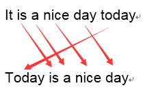
原文:今天天气不错
机器译文:It is a nice day today
人工译文:Today is a nice day
1−gram:
可以看到机器译文一共6个词,有5个词语都命中的了参考译文,P1=56
3−gram:
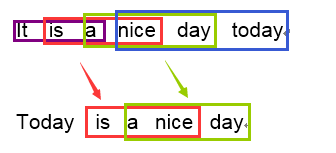
机器译文一共可以分为4个3−gram的词组,其中有2个可以命中参考译文,那么P3=24
Wn表示Pn的权重,一般为加权平均,即Wn=1N,其中N为gram的数量,一般不大于4
Recall-Oriented Understudy for Gisting Evaluation,可以看做是BLEU 的改进版,专注于召回率而非精度。换句话说,它会查看有多少个参考译句中的 n 元词组出现在了输出之中。
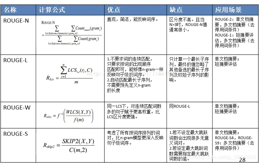
ROUGE大致分为四种(常用的是前两种): - ROUGE-N (将BLEU的精确率优化为召回率) - ROUGE-L (将BLEU的n-gram优化为公共子序列) - ROUGE-W (将ROUGE-L的连续匹配给予更高的奖励) - ROUGE-S (允许n-gram出现跳词(skip))
注意:
关于rouge包给出三个结果,而论文只有一个值,比如
1 | [{'rouge-1': {'r': 1.0, 'p': 1.0, 'f': 0.999999995}, 'rouge-2': {'r': 0.0, 'p': 0.0, 'f': 0.0}, 'rouge-l': {'r': 1.0, 'p': 1.0, 'f': 0.999999995}}] |
用“r”,recall就好了
https://blog.csdn.net/qq_36533552/article/details/107444391
https://zhuanlan.zhihu.com/p/144182853
https://arxiv.org/pdf/2006.14799.pdf
https://www.cnblogs.com/by-dream/p/7679284.html
https://blog.csdn.net/qq_30232405/article/details/104219396
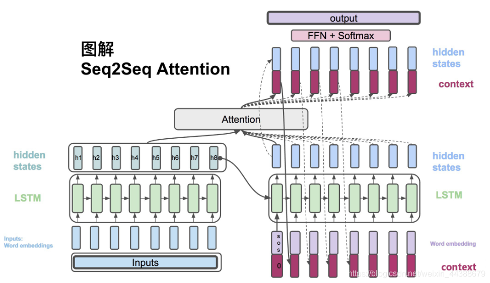
左边为encoder,对输入文本编码,右边为decoder,解码并应用。
整个流程的图解可以参考https://blog.csdn.net/weixin_44388679/article/details/102575223 中的“四、图解Attention Seq2Seq”,非常详细。
在训练阶段,如果使用Teacher Forcing策略,那么目标句子单词的word embedding使用真值,否则使用预测结果;至于预测阶段不能使用Teacher Forcing。
beam search本质为介于蛮力与贪心之间的策略。对于贪心,每一级的输出只选择top1的结果作为下一级输入,然后top1的结果只是局部最优,不一定是全局最优,精度可能较低。对于蛮力,每级将全部结果输入下级,假设L为词表大小,那么最后一级的数据量为Lm,m为decoder 的cell数量,计算效率太低。对于beam search,每级选择top k作为下级输入,综合了效率和精度。
0 为什么rnn based seq2seq不需要额外添加位置信息?
天然有位置信息(迭代顺序)
1 为什么rnn based seq2seq输入输出长度可变?
因为rnn based seq2seq是迭代进行的,所以长度可变
2 训练的时候要padding吗?
不用padding
https://zhuanlan.zhihu.com/p/47929039
人为构建,比较主观,不利于维护
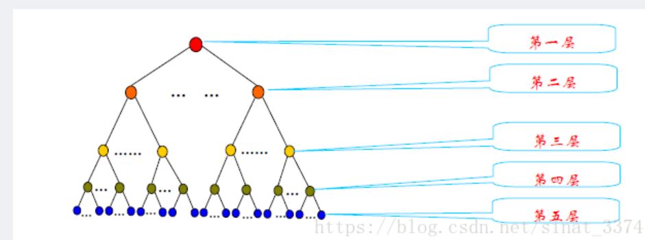
扩展版同义词词林分为5层结构,如图,随着级别的递增,词义刻画越来越细,到了第五层,每个分类里词语数量已经不大,很多只有一个词语,已经不可再分,可以称为原子词群、原子类或原子节点。不同级别的分类结果可以为自然语言处理提供不同的服务,例如第四层的分类和第五层的分类在信息检索、文本分类、自动问答等研究领域得到应用。有研究证明,对词义进行有效扩展,或者对关键词做同义词替换可以明显改善信息检索、文本分类和自动问答系统的性能。
下载后的词典文件如下所示:
1 | Aa01A01= 人 士 人物 人士 人氏 人选 |
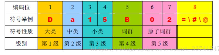
表中的编码位是按照从左到右的顺序排列。第八位的标记有3 种,分别是“=”、“#”、“@”, “=”代表“相等”、“同义”。末尾的“#”代表“不等”、“同类”,属于相关词语。末尾的“@”代表“自我封闭”、“独立”,它在词典中既没有同义词,也没有相关词。
源码如下
1 | class WordSimilarity2010(SimilarBase): |
环境准备:pip install WordSimilarity
1 | from word_similarity import WordSimilarity2010 |
1 | 联系方式 电话 相似度为 0 |
综合了词林cilin与知网hownet的相似度计算方法,采用混合策略,混合策略具体可以参考源码,如下
1 | from hownet.howNet import How_Similarity |
参考https://github.com/yaleimeng/Final_word_Similarity
1 | from Hybrid_Sim import HybridSim |
1 | 词林词汇量 77498 知网词汇量 53336 |
基于样本构建,利于维护
word2vec的原理和词向量获取过程不在此赘述,在本部分主要讲解基于word2vec的词向量如何计算词语相似度。源码如下
1 | def similarity(self, w1, w2): |
训练
1 | from gensim.models.word2vec import Word2Vec |
使用
1 | from gensim import models |
1 | 联系方式 电话 相似度为 -0.014857853 |
https://blog.csdn.net/sinat_33741547/article/details/80016713
https://arxiv.org/abs/1810.04805
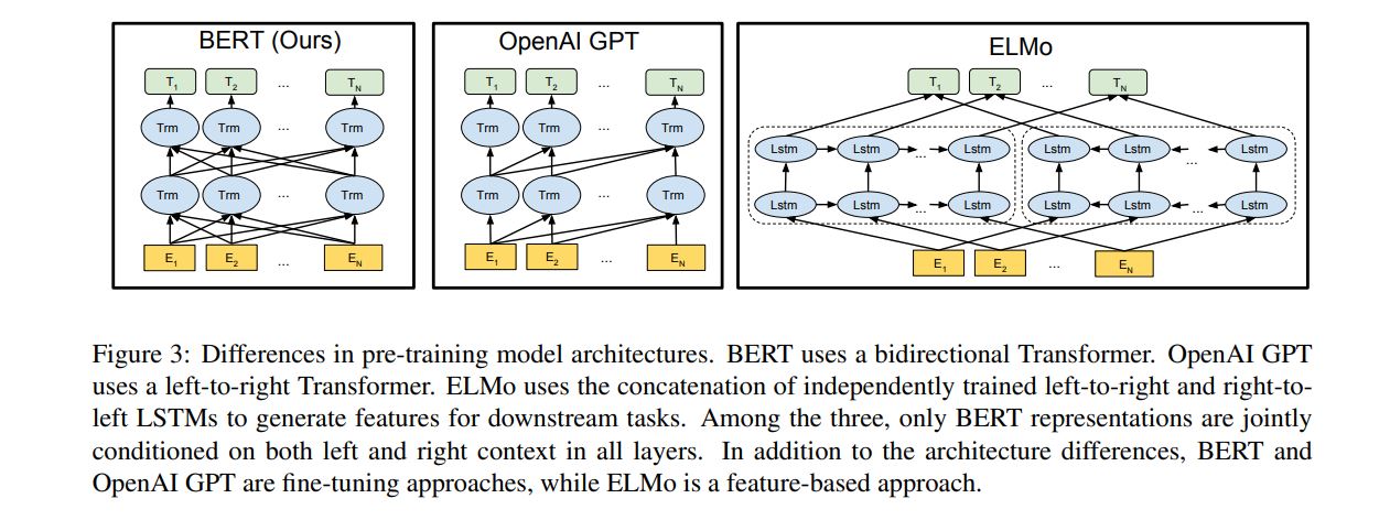
整体结构如上图,基本单元为Transformer 的encoder部分。作者对结构的描述为:BERT’s model architecture is a multi-layer bidirectional Transformer encoder。
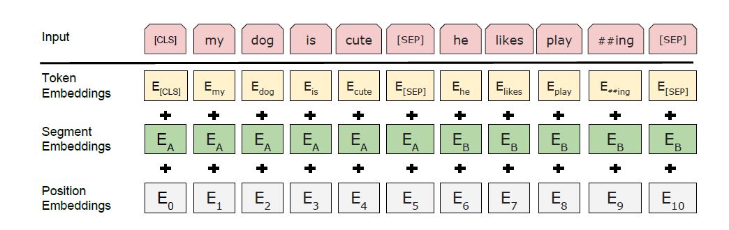
[CLS]表征句子开始,[SEP]表示句子结束以及分割两个句子
Token Embedding为词向量的表示,Position Embedding为位置信息,Segment Embedding表示A,B两句话,最后的输入向量为三者相加。比起transformer多一个Segment Embedding。
具体例子:https://www.cnblogs.com/d0main/p/10447853.html
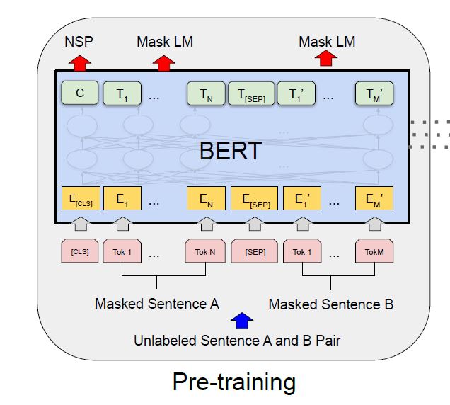
1 Masked LM
standard conditional language models can only be trained left-to-right or right-to-left , since bidirectional conditioning would allow each word to indirectly “see itself”.In order to train a deep bidirectional representation,MLM
The training data generator chooses 15% of the token positions at random for prediction. If the i-th token is chosen, we replace the i-th token with (1) the [MASK] token 80% of the time (2) a random token 10% of the time (3) the unchanged i-th token 10% of the time.
2 Next Sentence Prediction (NSP)
In order to train a model that understands sentence relationships
choosing the sentences A and B for each pretraining example, 50% of the time B is the actual next sentence that follows A (labeled as IsNext), and 50% of the time it is a random sentence from the corpus (labeled as NotNext).
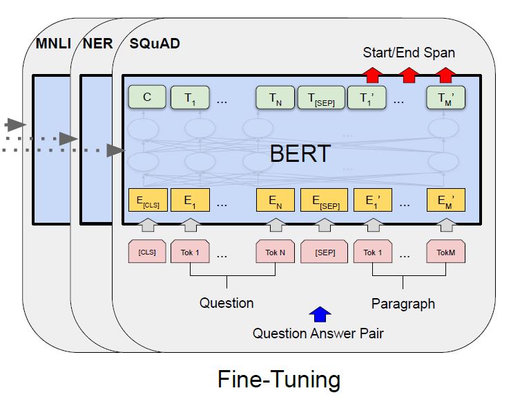
For each task, we simply plug in the task specific inputs and outputs into BERT and finetune all the parameters end-to-end.
输入: 可以为句子对或者单句,取决于特定任务
输出:At the output, the token representations are fed into an output layer for token level tasks, such as sequence tagging or question answering, and the [CLS] representation is fed into an output layer for classification, such as entailment or sentiment analysis.
1 bert为什么双向,gpt单向?
1.结构的不同
因为BERT用了transformer的encoder,在编码某个token的时候同时利用了其上下文的token,但是gptT用了transformer的decoder,只能利用上文
2.预训练任务的不同
2 为什么bert长度固定?
因为bert是基于transformer encoder的,不同位置的词语都是并行的,所以长度要提前固定,不可变
bert的输入输出长度为max_length,大于截断,小于padding,max_length的最大值为512
3 为什么bert需要补充位置信息?
因为是并行,不像迭代,没有天然的位置信息,需要补充position embedding。
对于中文和英文而言,由于语言差异导致算法也有差异。对于中文,存在字粒度和词粒度。对于英文,存在三个级别的粒度,character level,subword level,word level。下面主要阐述中文的词粒度和英文的subword level。
https://zhuanlan.zhihu.com/p/146792308
1 | # #####stanfordcorenlp |
1 | Tokenize: ['搜索', '引擎', '会', '通过', '日志', '文件', '把', '用户', '每次', '检索', '使用', '的', '所有', '检索', '串都', '记录', '下来'] |
观察结果,可以看出thulac分词效率最高,jieba分词的精度和效率比较平衡,stanfordcorenlp分词粒度很细,但是速度慢
SubWord算法如今已成为一个重要的NLP模型的提升算法。其主要优势如下:
1.word level存在OOV问题,一旦碰到就是back off to a dictionary,无法很好地处理未知和罕见词汇
2.Character level可以解决OOV,但是相比于 word-level , Character-level 的输入句子变长,使得数据变得稀疏,而且对于远距离的依赖难以学到,训练速度降低。
常见的SubWord算法有:BPE,WordPiece,Unigram Language Model等
全称为Byte Pair Encoding,算法来自paper《Neural Machine Translation of Rare Words with Subword Units》。
原理
注意,每次合并后词表可能出现3种变化:
例子:
训练语料为:
Iter 1, 最高频连续字节对”e”和”s”出现了6+3=9次,合并成”es”,输出:
Iter 2, 最高频连续字节对”es”和”t”出现了6+3=9次, 合并成”est”,输出:
Iter 3, 以此类推,最高频连续字节对为”est”和”</w>” ,合并后输出:
……
Iter n, 继续迭代直到达到预设的subword词表大小或下一个最高频的字节对出现频率为1。
代码
1 | import re, collections |
1 | ('e', 's') |
编码
1.将subword词表按照子词长度由大到小排序。
2.对于每个单词,遍历排好序的subword词表,寻找是否有token是当前单词的子字符串。最终,我们将迭代所有token,并将所有子字符串替换为token。
3.如果仍然有子字符串没被替换但所有token都已迭代完毕,则将剩余的子字符串替换为特殊token,如
例子:
1 | # 给定单词序列 |
编码的计算量很大。对于已知数据,我们可以pre-tokenize所有单词,并在词典中保存单词和tokenize的结果。如果存在字典中不存在的未知单词,可以应用上述编码方法对单词进行tokenize,然后将新单词以及tokenize的结果添加到字典中备用。
解码
将所有的subword拼在一起。
例子:
1 | # 编码序列 |
1.构建词表,假设有subword词表:[“errrr</w>”, “tain</w>”, “moun”, “est</w>”, “high”, “the</w>”, “a</w>”]
2.编码,词语”highest”编码成[“high”, “est</w>”]
3.向量表示,[Ehigh, Eest(/w)]]
https://www.cnblogs.com/d0main/p/10447853.html
算法来自于《Google’s Neural Machine Translation System: Bridging the Gap between Human and Machine Translation》
WordPiece算法可以看作是BPE的变种。不同点在于,WordPiece基于概率生成新的subword而不是下一最高频字节对。
https://arxiv.org/abs/1607.04606
《Neural Machine Translation with Byte-Level Subwords》
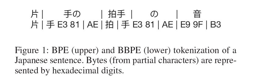
我们在进行中文NLP任务的时候,目前基本都是字粒度;英文的话大多数是使用subword的wordpiece。
https://zhuanlan.zhihu.com/p/112444056
https://arxiv.org/pdf/1508.07909.pdf
https://zhuanlan.zhihu.com/p/38130825
文本表示的表示形式可以是单一数值(基本没人用),可以是向量(目前主流),好奇有没有高纬tensor表示的?下文是基于向量表示的。
举个例子,有样本如下:
Jane wants to go to Shenzhen.
Bob wants to go to Shanghai.
基于上述两个文档中出现的单词,构建如下一个词典:
Vocabulary= [Jane, wants, to, go, Shenzhen, Bob, Shanghai]
那么wants 可以表示为
词向量模型是考虑词语位置关系的一种模型。通过大量语料的训练,将每一个词语映射到高维度的向量空间当中,使得语意相似的词在向量空间上也会比较相近,举个例子,如
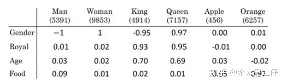
上表为词向量矩阵,其中行表示不同特征,列表示不同词,Man可以表示为
性质:embMan−embWomen≈embKing−embQueen
常见的词向量矩阵构建方法有,word2vec,GloVe
词袋模型不考虑文本中词与词之间的上下文关系,仅仅只考虑所有词的权重。而权重与词在文本中出现的频率有关。
例句:
Jane wants to go to Shenzhen.
Bob wants to go to Shanghai.
基于上述两个文档中出现的单词,构建如下一个词典:
Vocabulary= [Jane, wants, to, go, Shenzhen, Bob, Shanghai]
那么上面两个例句就可以用以下两个向量表示,其值为该词语出现的次数:
SentEval is a popular toolkit to evaluate the quality of sentence embeddings.
sentence BERT
BERT-flow
https://zhuanlan.zhihu.com/p/444346578
https://zhuanlan.zhihu.com/p/353187575
由于Bag of words不考虑词语的顺序,因此引入bag of n-gram。针对英文,词内的是char n-gram,用于词向量;词之间的是word n-gram,用于分类;对于中文,存在词粒度和字粒度。
举个例子,句子A为”今天天气真不错”,这里以词粒度举例,先分词为[“今天”,”天气”,”真“,”不错“]
uni-gram:今天 天气 真 不错
2-gram为:今天/天气 天气/真 真/不错
3-gram为:今天/天气/真 天气/真/不错
由于n-gram的量远比word大的多,完全存下所有的n-gram也不现实。FastText采用了hashing trick的方式,如下图所示:
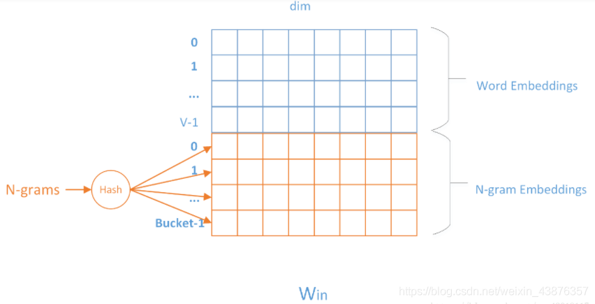
用哈希的方式既能保证查找时O(1)的效率,又可能把内存消耗控制在O(buckets * dim)范围内。不过这种方法潜在的问题是存在哈希冲突,不同的n-gram可能会共享同一个embedding。如果buckets取的足够大,这种影响会很小。
代码如下:
1 | def build_dataset(config, ues_word): |
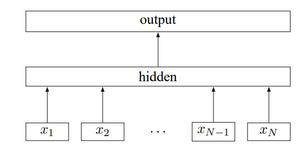
模型结构上word2vec的cbow模型很像
输入层:举个例子,输入文本”今天天气真不错”,词粒度的2-gram为
x2=[emb今天/天气,emb天气/真,emb真/不错],emb为词向量矩阵x1,x2,...,xN最后输入到中间层的形式为:mean([x1x2...xN]),其中mean为对每个x的列求平均中间层:线形层+relu作为激活函数
输出层:为简单的线形层
代码:
1 | class Model(nn.Module): |
对于分类问题,神经网络的输出结果需要经过softmax将其转为概率分布后才可以利用交叉熵计算loss
由于普通softmax的计算效率比较低,计算效率为O(Kd)使用分层的softmax时间复杂度可以达到dlogK,K为分类的数量,d为向量的维度
假设输出为Ypred=[y1,y2,…,yK],则Pyi为
Pyi=eyi∑Kj=0eyj其中yi的维度为d,从公式可以看出计算效率为O(Kd)
霍夫曼树可以参考 https://zhuanlan.zhihu.com/p/154356949
为什么要霍夫曼,普通的不行?
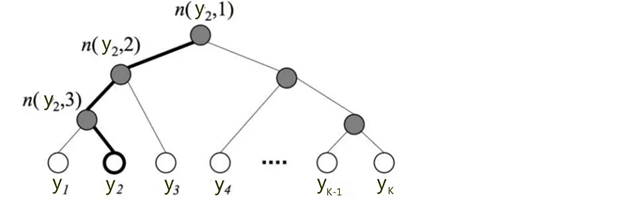
分层softmax核心思想为利用训练样本构建霍夫曼树,如下
树的结构是根据不同类在样本中出现的频次构造的,即频次越大的节点距离根节点越近。K个不同的类组成所有的叶子节点,K−1个内部节点作为参数。从根节点到某个叶子节点yi经过的节点和边形成一条路径,路径长度表示为 Lyi,n(yi,j)表示路径上的节点,那么
Pyi=Lyi∏j=1P(n(yi,j),left or right)=Lyi−1∏j=0σ(f(n(yi,j+1)==LC(n(yi,j)))θTn(yi,j)Y)其中LC(n(yi,j)表示n(yi,j)的左孩子,σ为SIGMOD函数,f(m)={1if m==true−1 else从公式可以看出时间复杂度降低至dlogK。
以图中y2为例:
Py2=P(n(y2,1),left)⋅P(n(y2,2),left)⋅P(n(y2,3),right)=σ(θTn(y2,1)Y)⋅σ(θTn(y2,2)Y)⋅σ(−θTn(y2,3)Y)从根节点走到叶子节点 y2 ,实际上是在做了3次逻辑回归。
https://arxiv.org/abs/1607.04606
https://arxiv.org/abs/1607.01759
https://zhuanlan.zhihu.com/p/32965521
https://blog.csdn.net/qq_27009517/article/details/80676022
http://alex.smola.org/papers/2009/Weinbergeretal09.pdf
https://arxiv.org/abs/1607.04606
fasttext工具 https://github.com/facebookresearch/fastText
1.We propose a new simple network architecture, the Transformer, based solely on attention mechanisms, dispensing with recurrence and convolutions entirely.
2.Experiments on two machine translation tasks show these models to be superior in quality while being more parallelizable and requiring significantly less time to train.
![]()
in order for the model to make use of the order of the sequence, we must inject some information about the relative or absolute position of the tokens in the sequence. There are many choices of positional encodings, learned and fixed [9]. In this work, we use sine and cosine functions of different frequencies:
PE(pos,2i)=sin(pos/100002i/dmodel)PE(pos,2i+1)=cos(pos/100002i/dmodel)详细可参考 https://wmathor.com/index.php/archives/1453/
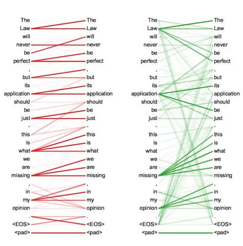
其中不同颜色表示不同head,颜色深浅表示词的关联程度。
不同head表示不同应用场景 ,单一head表示某个场景下,各个字之间的关联程度
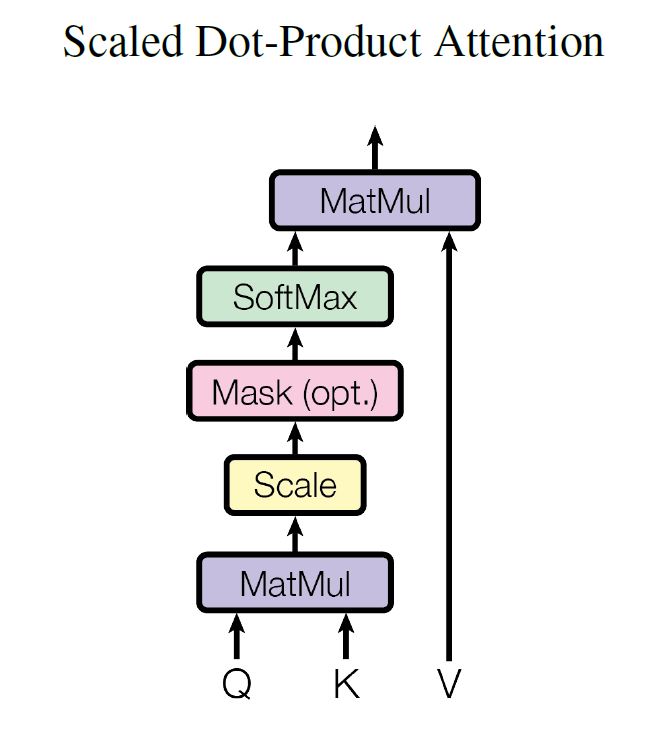
dk : keys of dimension
为什么scale?We suspect that for large values of dk, the dot products grow large in magnitude, pushing the softmax function into regions where it has extremely small gradients.
Mask
可以分为两类:Attention Mask和Padding Mask,接下来具体讲解。
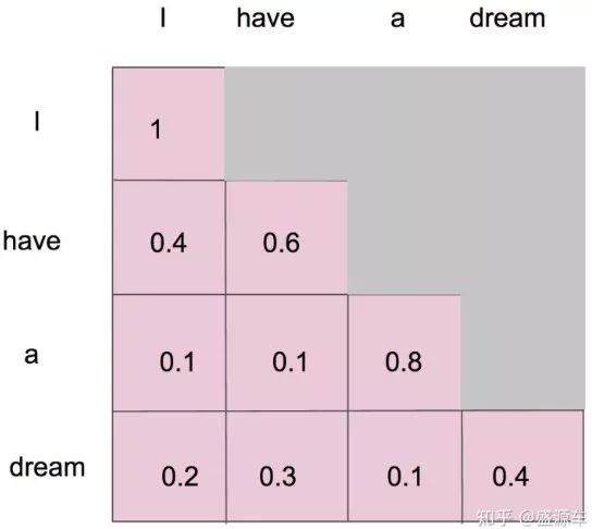
1.Attention Mask
ensures that the predictions for position i can depend only on the known outputs at positions less than i.
sotfmax前要mask,上三角mask掉
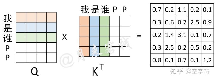
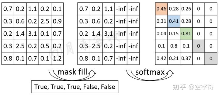
2.Padding Mask
Padding位置上的信息是无效的,所以需要丢弃。
过程如下图示:
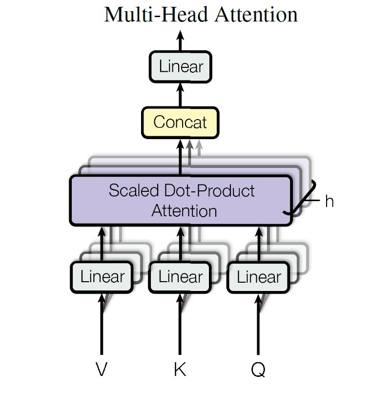
Multi-head attention allows the model to jointly attend to information from different representation subspaces at different positions.
MultiHead(Q,K,V)=Concat(head1,...,headn)WOwhere headi=Attetion(QWQi,kWKi,VWVi)1.encoder-decoder attention layers
结构:queries come from the previous decoder layer,and the memory keys and values come from the output of the encoder.
目的:This allows every position in the decoder to attend over all positions in the input sequence.
2.encoder contains self-attention layers
结构:keys, values and queries come from the same place
目的:Each position in the encoder can attend to all positions in the previous layer of the encoder.
3.self-attention layers in the decoder
结构:keys, values and queries come from the same place
目的:allow each position in the decoder to attend to all positions in the decoder up to and including that position
1).Input Embedding与Positional Encoding
X=Input Embedding+Positional Encoding2). multi-head attention
Q=Linearq(X)=XWQK=Lineark(X)=XWKV=Linearv(X)=XWVXattention=Attention(Q,K,V)3). 残差连接与 Layer Normalization
Xattention=X+XattentionXattention=LayerNorm(Xattention)4). FeedForward
Xhidden=Linear(ReLU(Linear(Xattention)))5). 残差连接与 Layer Normalization
Xhidden=Xattention+XhiddenXhidden=LayerNorm(Xhidden)其中$ X_{hidden} \in \mathbb{R}^{batch_size \ \ seq_len \ \ embed_dim} $
我们先从 HighLevel 的角度观察一下 Decoder 结构,从下到上依次是:
1 并行化
训练encoder,decoder都并行,测试encoder并行,decoder不是并行
https://zhuanlan.zhihu.com/p/368592551
2 self-attention和普通attention的区别
取决于query和key是否在一个地方
3 Why Self-Attention
Motivating our use of self-attention we consider three desiderata.
1.One is the total computational complexity per layer.
2.Another is the amount of computation that can be parallelized, as measured by the minimum number of sequential operations required.
3.The third is the path length between long-range dependencies in the network