原文地址 https://cseweb.ucsd.edu/classes/fa17/cse291-b/reading/Rendle2010FM.pdf

https://zhuanlan.zhihu.com/p/50426292

a new model class that combines the advantages of Support Vector Machines (SVM) with factorization models

I. INTRODUCTION

In total, the advantages of our proposed FM are:
1) FMs allow parameter estimation under very sparse data where SVMs fail.
2) FMs have linear complexity, can be optimized in the primal and do not rely on support vectors like SVMs.
3) FMs are a general predictor that can work with any real valued feature vector.

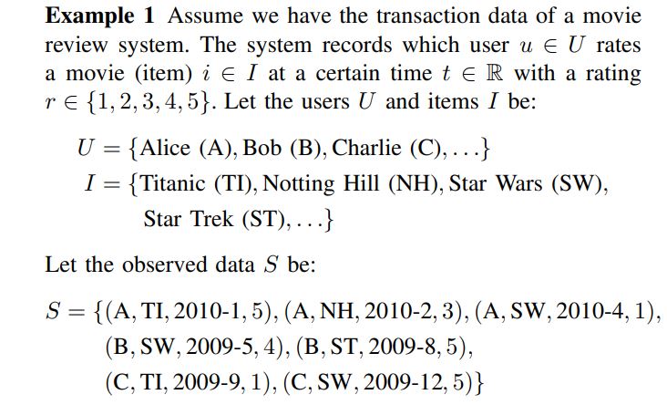
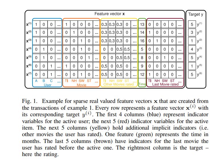
II. PREDICTION UNDER SPARSITY

III. FACTORIZATION MACHINES (FM)

A. Factorization Machine Model

1) 模型:

$x_i$表示第$i$个特征，但是针对上式，一个很大的问题，用户交互矩阵往往是比较稀疏的，这样就会导致对$w_{i,j}$的估算存在很大的问题。举个例子，假如想要估计Alice(A)和Star Trek(ST)的交互参数$w_{A,ST}$，由于训练集中没有实例同时满足$x_A$和$x_{ST}$非零，这会造成$w_{A,ST}=0$。因此这里使用了矩阵分解的思想：

2) 提升效率:

直接计算上面的公式求解$\hat{y}(x)$的时间复杂度为$O ( k n^2 ) $，因为所有的特征交叉都需要计算。但是可以通过公式变换，将时间复杂度减少到$O(kn)$，如下公式推导

B. Factorization Machines as Predictors

FM can be applied to a variety of prediction tasks. Among them are: Regression，Binary classification，Ranking

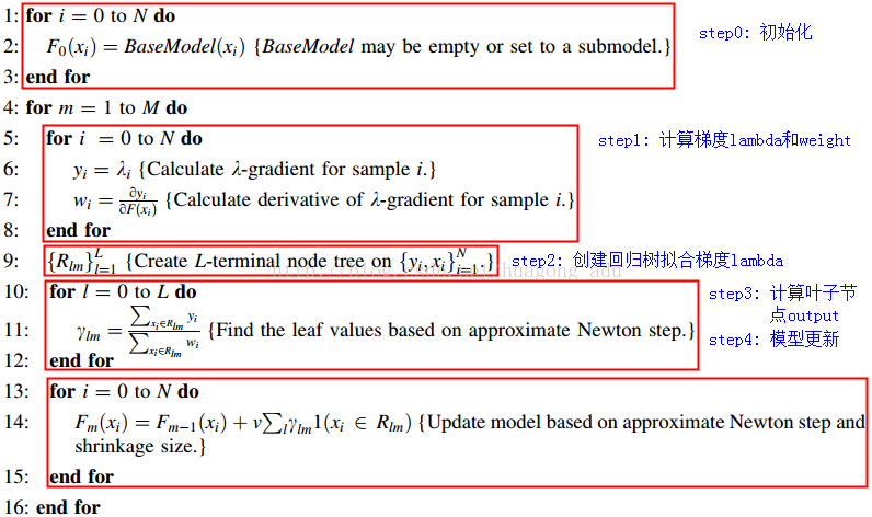
C. Learning Factorization Machines

the model parameters of FMs can be learned efficiently by gradient descent methods – e.g. stochastic gradient descent (SGD).The gradient of the FM model is:

D. d-way Factorization Machine

The 2-way FM described so far can easily be generalized to a d-way FM:

直接计算上式的时间复杂度为$O(k_dn^d)$，利用类似上面的公式变形也可以将其降低为$O(k_d n )$

E. Summary

FMs model all possible interactions between values in the feature vector $x$ using factorized interactions instead of full parametrized ones. This has two main advantages:

1) The interactions between values can be estimated even under high sparsity. Especially, it is possible to generalize to unobserved interactions.
2) The number of parameters as well as the time for prediction and learning is linear.

IV. FMS VS. SVMS

V. FMS VS. OTHER FACTORIZATION MODELS

参考

https://blog.csdn.net/qq_26822029/article/details/103993243

What are sparse features?

Features with sparse data are features that have mostly zero values. This is different from features with missing data.

Why is machine learning difficult with sparse features?

Common problems with sparse features include:

1. If the model has many sparse features, it will increase the space and time complexity of models. Linear regression models will fit more coefficients, and tree-based models will have greater depth to account for all features.
2. Model algorithms and diagnostic measures might behave in unknown ways if the features have sparse data. Kuss [2002] shows that goodness-of-fit tests are flawed when the data is sparse.
3. If there are too many features, models fit the noise in the training data. This is called overfitting. When models overfit, they are unable to generalize to newer data when they are put in production. This negatively impacts the predictive power of models.
4. Some models may underestimate the importance of sparse features and given preference to denser features even though the sparse features may have predictive power. Tree-based models are notorious for behaving like this. For example, random forests overpredict the importance of features that have more categories than those features that have fewer categories.

Methods for dealing with sparse features

1. Removing features from the model

2. Make the features dense

3. Using models that are robust to sparse features

参考

https://www.kdnuggets.com/2021/01/sparse-features-machine-learning-models.html#:~:text=%20Methods%20for%20dealing%20with%20sparse%20features%20,that%20are%20robust%20to%20sparse%20features%20More%20

google继lasertagger之后的又一篇text edit paper

In contrast to conventional sequence-to-sequence (seq2seq) models, FELIX is efficient in low-resource settings and fast at inference time, while being capable of modeling flexible input-output transformations. We achieve this by decomposing the text-editing task into two sub-tasks: tagging to decide on the subset of input tokens and their order in the output text and insertion to in-fill the missing tokens in the output not present in the input.

1 Introduction

In particular, we have designed FELIX with the following requirements in mind: Sample efficiency, Fast inference time, Flexible text editing

2 Model description

FELIX decomposes the conditional probability of generating an output sequence $y$ from an input
$x$ as follows:

2.1 Tagging Model

trained to optimize both the tagging and pointing loss:

Tagging :

tag sequence $\textbf{y}^t$由3种tag组成：$KEEP$，$DELETE$，$INSERT (INS)$

Tags are predicted by applying a single feedforward layer $f$ to the output of the encoder $\textbf{h}^L$ (the source sentence is first encoded using a 12-layer BERT-base model). $\textbf{y}^t_i=argmax(f(\textbf{h}^L_i))$

Pointing:

Given a sequence $\textbf{x}$ and the predicted tags $\textbf{y}^t$ , the re-ordering model generates a permutation $\pi$ so that from $\pi$and $\textbf{y}^t$ we can reconstruct the insertion model input $\textbf{y}^m$. Thus we have:

Our implementation is based on a pointer network. The output of this model is a series of predicted pointers (source token → next target token)

The input to the Pointer layer at position $i$:

其中$e(\textbf{y}_i^t)$is the embedding of the predicted tag，$e(\textbf{p}_i)$ is the positional embedding

The pointer network attends over all hidden states, as such:

其中$\textbf{h}_i^{L+1}$ as $Q $, $\textbf{h}_{\pi(i)}^{L+1}$ as $K$

When realizing the pointers, we use a constrained beam search

2.2 Insertion Model

To represent masked token spans we consider two options: masking and infilling. In the former case the tagging model predicts how many tokens need to be inserted by specializing the $INSERT$ tag into $INS_k$, where $k$ translates the span into $ k$ $MASK$ tokens. For the infilling case the tagging model predicts a generic $INS$ tag.

Note that we preserve the deleted​ span in the input to the insertion model by enclosing it between $[REPL]$ and $[/REPL]$ tags.

our insertion model is also based on a 12-layer BERT-base and we can directly take advantage of the BERT-style pretrained checkpoints.

参考

https://aclanthology.org/2020.findings-emnlp.111.pdf

https://arxiv.org/pdf/2106.09297.pdf

http://xtf615.com/2021/10/07/taobao-ebr/

1.INTRODUCTION

框架是搜索系统主流的结构，即匹配/检索，粗排，精排，重排。

2.RELATED WORK

2.1 Deep Matching in Search

fall into two categories: representation-based learning and interaction-based learning.

Other than semantic and relevance matching, more complex factors/trade-offs, e.g., user personalization [2, 3, 10] and retrieval efficiency [5], need to be considered when applying deep models to a large-scale online retrieval system.

2.2 Deep Retrieval in Industry Search

Representation-based models with an ANN (approximate near neighbor) algorithm have become the mainstream trend to efficiently deploy neural retrieval models in industry.

3 MODEL

整体结构入下：

3.1 Problem Formulation

$\mathcal{U}=\{u_1,…,u_u,…u_N\}$表示$N$个用户，$\mathcal{Q}=\{q_1,…,q_u,…q_N\}$表示与用户对应的$N$个query，$\mathcal{I}=\{i_1,…,i_u,…i_M\}$表示$M$个商品。将用户$u$的历史行为根据时间分成3个部分：1.real-time，before
the current time step，$\mathcal{R}^u=\{i_1^u,…,i_t^u,…i_T^u\}$ 2.short-term, before $\mathcal{R}$ and within ten days,$\mathcal{S}^u=\{i_1^u,…,i_t^u,…i_T^u\}$ 3.long-term sequences,before $\mathcal{S}$ and within one month,$\mathcal{L}^u=\{i_1^u,…,i_t^u,…i_T^u\}$ ，$T$为时间长度。任务可以定义为：

其中$\mathcal{F}(\cdot),\phi(\cdot),\varphi(\cdot)$分别表示scoring function, query and behaviors encoder, and item encoder

3.2 User Tower

3.2.1 Multi-Granular Semantic Unit

挖掘query的语义，原始输入包含当前query和历史query

没有说明为什么这么设计，感觉就是工程试验的结论。有个疑问，直接用BERT等深度语言模型来挖掘query的语义不好吗？

query表示为$q_u=\{w_1^u,…,w_n^u\}$,例如{红色，连衣裙}，$w_u=\{c_1^u,…,c_m^u\}$,例如{红，色}，history query表示为$q_{his}=\{q_1^u,…,q_k^u\} $,例如{绿色，半身裙，黄色，长裙}，其中$w_n \in \mathbb{R}^{1\times d},c_m \in \mathbb{R}^{1\times d},q_k \in \mathbb{R}^{1\times d}$

其中𝑇𝑟𝑚,𝑚𝑒𝑎𝑛_𝑝𝑜𝑜𝑙𝑖𝑛𝑔, and 𝑐𝑜𝑛𝑐𝑎𝑡 denote the Transformer ,average, and vertical concatenation operation, respectively

3.2.2 User Behaviors Attention

其中$W_f$是embedding matrix，$x_i^{f}$是one-hot vector, $\mathcal{F}$是side information (e.g., leaf category, first-level category, brand and,shop)

real-time sequences

User’s click_item

short-term sequences

User’s click_item

long-term sequence

$\mathcal{L}^u$由四个部分构成，分别为$\mathcal{L}^{u}_{item},\mathcal{L}^{u}_{shop},\mathcal{L}^{u}_{leaf},\mathcal{L}^{u}_{brand}$,每个部分包含3个动作，分别为click，buy，collect。

3.2.3 Fusion of Semantics and Personalization

3.3 Item Tower

For the item tower, we experimentally use item ID and title to obtain the item representation 𝐻𝑖𝑡𝑒𝑚.Given the representation of item 𝑖’s ID, $e_i \in \mathbb{R}^{1\times d}$ , and its title segmentation result $T_i=\{w_1^{i},…,w_N^{i}\}$

where $W_t$ is the transformation matrix. We empirically find that applying LSTM [12] or Transformer [27] to capture the context of the title is not as effective as simple mean-pooling since the title is stacked by keywords and lacks grammatical structure.

3.4 Loss Function

adapt the softmax cross-entropy loss as the training objective

where $\mathcal{F},I,i^+,q_u$denote the inner product, the full item pool, the item tower’s representation $H_{item}$, and the user tower’s representation $H_{qu}$, respectively.

3.4.1 Smoothing Noisy Training Data

the softmax function with the temperature parameter $\tau$ is defined as follows

If 𝜏->0, the fitted distribution is close to one hot distribution,If 𝜏->∞, the fitted distribution is close to a uniform distribution

3.4.2 Generating Relevance-improving Hard Negative Samples

We first select the negative items of $i^-$ that have the top-𝑁 inner product scores with $q_u $ to form the hard sample set $I_{hard}$

其中$\alpha\in \mathbb{R}^{N\times1}$is sampled from the uniform distribution 𝑈 (𝑎, 𝑏) (0 ≤ 𝑎 < 𝑏 ≤ 1).

1.RankNet

RankNet采用pairwise的方法进行模型训练。

loss推导

给定特定$query$下的两个文档$U_i$和$U_j$，其特征向量分别为$x_i$和$x_j$，经过RankNet进行前向计算得到对应的分数为$s_i=f(x_i)$和$s_j=f(x_j)$。用$U_i \rhd U_j$表示$U_i$比$U_j$排序更靠前。继而可以用下面的公式来表示$U_i$应该比$U_j$排序更靠前的概率：

定义$S_{ij} \in \{0,\pm1\}$为文档$i$和文档$j$被标记的标签之间的关联，即

定义$\overline{P}_{ij}=\frac{1}{2}(1+S_{ij})$表示$U_i$应该比$U_j$排序更靠前的已知概率，则可以用交叉熵定义优化目标的损失函数：

注意：$\sigma$是超参数

ranknet 加速

2.LambdaRank

ranket缺陷为只考虑pair的相对位置没有考虑二者在列表的整体位置

LambdaRank本质为ranknet基础上加入Listwise的指标，因此有人将LambdaRank归为listwise方法，也有归到pairwise方法

2.1 RankNet的局限

2.2 LambdaRank定义

上述公式可以进一步简化，即只考虑$S_{ij}=1$ （为什么可以？？？？？）

那么Lambda，$\lambda$，就是梯度

为了加强排序中前后顺序的重要性，Lambda在原基础上引入评价指标Z（如NDCG），把交换两个文档的位置引起的评价指标的变化$|\Delta Z_{ij}|$作为其中一个因子：

反推出 LambdaRank 的损失函数：

3.LambdaMART

属于listwise，也有说pairwise。

LambdaMART=lambda($\lambda$)+mart(gbdt)

$\lambda$就是梯度，lambdarank就是一种loss，gbdt就是模型

lambdamart说白了就是利用gbdt计算lambdarank中s，或者说将lambdarank作为gbdt的loss

gbdt，lambdamart算法流程差异在于step1

GBDT：

1. 初始化： $f_0(x) = \mathop{\arg\min}\limits_\gamma \sum\limits_{i=1}^N L(y_i, \gamma)$
2. for m=1 to M:
   (a). 计算负梯度： $\tilde{y}_i = -\frac{\partial L(y_i,f_{m-1}(x_i))}{\partial f_{m-1}(x_i)}, \qquad i = 1,2 \cdots N$
   (b). $\left \{ R_{jm} \right\}_1^J = \mathop{\arg\min}\limits_{\left \{ R_{jm} \right\}_1^J}\sum\limits_{i=1}^N \left [\tilde{y}_i - h_m(x_i\,;\,\left \{R_{jm},b_{jm} \right\}_1^J) \right]^2$
   (c). $\gamma_{jm} = \mathop{\arg\min}\limits_\gamma \sum\limits_{x_i \in R_{jm}}L(y_i,f_{m-1}(x_i)+\gamma)$
   (d). $f_m(x) = f_{m-1}(x) + \sum\limits_{j=1}^J \gamma_{jm}I(x \in R_{jm})$
3. 输出$f_M(x)$

LambdaMART:

参考

https://blog.csdn.net/laolu1573/article/details/87372514

https://liam.page/uploads/slides/lambdamart.pdf

https://blog.csdn.net/zpalyq110/article/details/79527653

https://zhuanlan.zhihu.com/p/86354141

https://www.cnblogs.com/genyuan/p/9788294.html

https://blog.csdn.net/huagong_adu/article/details/40710305

https://zhuanlan.zhihu.com/p/270608987

https://www.cnblogs.com/bentuwuying/p/6690836.html

paper原文： https://www.microsoft.com/en-us/research/wp-content/uploads/2016/02/MSR-TR-2010-82.pdf

https://www.jianshu.com/p/a78b3f52c221

https://blog.csdn.net/zhoujialin/article/details/46697409

https://blog.csdn.net/w28971023/article/details/45849659

https://zhuanlan.zhihu.com/p/270608987

分类：

单调栈也分为单调递增栈和单调递减栈

• 单调递增栈：单调递增栈就是从栈底到栈顶数据是从大到小
• 单调递减栈：单调递减栈就是从栈底到栈顶数据是从小到大

举例：单调递增栈

现在有一组数10，3，7，4，12。从左到右依次入栈，则如果栈为空或入栈元素值小于栈顶元素值，则入栈；否则，如果入栈则会破坏栈的单调性，则需要把比入栈元素小的元素全部出栈。

10入栈时，栈为空，直接入栈，栈内元素为10。

3入栈时，栈顶元素10比3大，则入栈，栈内元素为10，3。

7入栈时，栈顶元素3比7小，则栈顶元素出栈，此时栈顶元素为10，比7大，则7入栈，栈内元素为10，7。

4入栈时，栈顶元素7比4大，则入栈，栈内元素为10，7，4。

12入栈时，栈顶元素4比12小，4出栈，此时栈顶元素为7，仍比12小，栈顶元素7继续出栈，此时栈顶元素为10，仍比12小，10出栈，此时栈为空，12入栈，栈内元素为12。

伪代码

1
2
3
4
5
6
7
8
9
10
11
12
13
14
15
16
17
18

stack<int> st;
//单调递增栈
for (遍历这个数组)
{
	if (栈空 || 栈顶元素大于等于当前比较元素)
	{
		入栈;
	}
	else
	{
		while (栈不为空 && 栈顶元素小于当前元素)
		{
			栈顶元素出栈;
			更新结果;
		}
		当前数据入栈;
	}
}

应用：

主要用于$O(n)$ 解决NGE问题（Next Greater Element）

• 比当前元素更大的下一个元素
• 比当前元素更大的前一个元素
• 比当前元素更小的下一个元素
• 比当前元素更小的前一个元素

参考

https://blog.csdn.net/lucky52529/article/details/89155694

GBDT （Gradient Boosting Decison Tree）=Gradient Boosting+cart回归树

注意是cart回归树，不是cart分类树

说白了就是gradient boosting基学习器为cart回归树

gradient boosting算法流程:

1.初始化：$f_0(x) = \mathop{\arg\min}\limits_\gamma \sum\limits_{i=1}^N L(y_i, \gamma)$

2.for m=1 to M:
(a). 计算负梯度： $\tilde{y}_i = -\frac{\partial L(y_i,f_{m-1}(x_i))}{\partial f_{m-1}(x_i)}, \quad i = 1,2 \cdots N$
(b). 通过最小化平方误差，用基学习器$h_m(x)$拟合$\tilde{y_i}$，$w_m = \mathop{\arg\min}\limits_w \sum\limits_{i=1}^{N} \left[\tilde{y}_i - h_m(x_i\,;\,w) \right]^2$
(c). 使用line search确定步长$ρ_m$，使$L$最小，$\rho_m = \mathop{\arg\min}\limits_{\rho} \sum\limits_{i=1}^{N} L(y_i,f_{m-1}(x_i) + \rho h_m(x_i\,;\,w_m))$
(d). $f_m(x) = f_{m-1}(x) + \rho_m h_m(x\,;\,w_m)$

3.输出$f_M(x)$

GBDT算法流程：

1. 初始化： $f_0(x) = \mathop{\arg\min}\limits_\gamma \sum\limits_{i=1}^N L(y_i, \gamma)$
2. for m=1 to M:
   (a). 计算负梯度： $\tilde{y}_i = -\frac{\partial L(y_i,f_{m-1}(x_i))}{\partial f_{m-1}(x_i)}, \qquad i = 1,2 \cdots N$
   (b). $\left \{ R_{jm} \right\}_1^J = \mathop{\arg\min}\limits_{\left \{ R_{jm} \right\}_1^J}\sum\limits_{i=1}^N \left [\tilde{y}_i - h_m(x_i\,;\,\left \{R_{jm},b_{jm} \right\}_1^J) \right]^2$
   (c). $\gamma_{jm} = \mathop{\arg\min}\limits_\gamma \sum\limits_{x_i \in R_{jm}}L(y_i,f_{m-1}(x_i)+\gamma)$
   (d). $f_m(x) = f_{m-1}(x) + \sum\limits_{j=1}^J \gamma_{jm}I(x \in R_{jm})$
3. 输出$f_M(x)$

参考

https://blog.csdn.net/zpalyq110/article/details/79527653

https://zhuanlan.zhihu.com/p/86354141

推导过程

Gradient Boosting为boosting算法的一种，采用和AdaBoost同样的加法模型，在第m次迭代中，前m-1个基学习器都是固定的，即

核心思想是得到基学习器$h_m(x)$和权重$p_m$

参数空间的梯度下降很常见，即

若将$f(x)$当成参数，则同样可以使用函数空间的梯度下降法：

对比（1）（2），我们发现$h_m(x) \approx -\frac{\partial L(y,f_{m-1}(x))}{\partial f_{m-1}(x)}$

算法流程:

1.初始化：$f_0(x) = \mathop{\arg\min}\limits_\gamma \sum\limits_{i=1}^N L(y_i, \gamma)$

2.for m=1 to M:
(a). 计算负梯度： $\tilde{y}_i = -\frac{\partial L(y_i,f_{m-1}(x_i))}{\partial f_{m-1}(x_i)}, \quad i = 1,2 \cdots N$
(b). 通过最小化平方误差，用基学习器$h_m(x)$拟合$\tilde{y_i}$，$w_m = \mathop{\arg\min}\limits_w \sum\limits_{i=1}^{N} \left[\tilde{y}_i - h_m(x_i\,;\,w) \right]^2$
(c). 使用line search确定步长$ρ_m$，使$L$最小，$\rho_m = \mathop{\arg\min}\limits_{\rho} \sum\limits_{i=1}^{N} L(y_i,f_{m-1}(x_i) + \rho h_m(x_i\,;\,w_m))$
(d). $f_m(x) = f_{m-1}(x) + \rho_m h_m(x\,;\,w_m)$

3.输出$f_M(x)$

参考

https://www.cnblogs.com/zhubinwang/p/5170087.html

https://www.cnblogs.com/massquantity/p/9174746.html

1.概述

基本上决策树都是二叉树

两幅图意思一样

2.决策树 vs 逻辑回归

最大的差异上图就可以看出，左边为逻辑回归的决策面，右边为决策树的决策面

3.构建算法

常见方法的有ID3，C4.5，CART，总结如下

3.1 ID3

假设训练数据集为 $D$,∣$D∣$表示其大小。设有$K$个分类$ C_1,C_2,…,C_K$。设特征集为$\textbf{A}$,假设某个特征$ A$ 有$ n$ 个不同的取值 $\{a_1,a_2,…,a_n\}$,根据特征$A$的取值将 $D$ 划分成$n$个子集。记子集 $D_i$中属于类$ C_k$的样本集合为 $D_{ik}$。

数据集$D$的经验熵$H(D)$:

特征$A$对数据集$ D$的经验条件熵$H(D|A)$

信息增益$g(D,A)$

算法流程:

1. 若$D$中所有实例都属于同一类 $C_k$,则 $T$ 为单节点树,并将类 $C_k$作为该节点的类标记,返回$T$.
2. 若$\textbf{A}=\phi$,则$T$为单节点树,并将$D$中实例最大的类$C_k$作为该节点的类标记,返回$T$.
3. 否则,按照信息增益的算法,计算每个特征对$D$的信息增益,取信息增益最大的特征 $A_g$.
4. 如果$A_g< \varepsilon$,则置 $T$为单节点树,并将$D$中实例最大的类$C_k$作为该节点的类标记,返回$T$.
5. 否则,对$A_g$的每一可能值 $a_i$,依$A_g=a_i$将$D$分成若干非空子集$D_i$
6. 以$D_i$为训练集,以$\textbf{A}- A_g $为特征集,递归地调用步骤1到步骤5,得到子树 $T_i$,全部 $T_i$构成$T$,返回$T$.

3.2 C4.5

 C4.5算法流程与ID3相类似，只不过将信息增益改为信息增益比，以解决偏向取值较多的属性的问题，另外它可以处理连续型属性。

分裂信息 $SplitInformation(D,A)$

信息增益比 $GainRatio(D, A)$

3.3 CART

3.3.1 CART分类树

CART分类树算法使用基尼系数来代替信息增益（比），基尼系数代表了模型的不纯度，基尼系数越小，不纯度越低，特征越好。这和信息增益（比）相反。

对于样本$D$，个数为$|D|$，假设$K$个类别，第$k$个类别的数量为$|C_k|$，则样本$D$的基尼系数表达式：

对于样本$D$，个数为$|D|$，根据特征$A$的某个值$a$，把$D$分成$|D_1|$和$|D_2|$，则在特征$A=a$的条件下，样本$D$的基尼系数表达式为：

算法流程：算法输入训练集$D$，基尼系数的阈值，样本个数阈值。输出的是决策树$T$。

(1)、对于当前节点的数据集为$D$，如果样本个数小于阈值或没有特征，则当前节点停止递归，返回决策树。

(2)、计算样本集$D$的基尼系数，如果基尼系数小于阈值，则当前节点停止递归，返回决策树。

(3)、计算当前节点所有特征的各个特征值对数据集$D$的基尼系数

(4)、在计算出来的所有基尼系数中，选择基尼系数最小的特征$A$和对应的特征值$a$，并把数据集划分成两部分$D_1$和$D_2$，同时建立当前节点的左右节点，左节点的数据集$D$为$D_1$，右节点的数据集$D$为$D_2$。

(5)、对左右的子节点递归的调用1-4步，生成决策树。

3.3.2 CART回归树

对回归树用平方误差最小化准则

算法流程：输入为训练数据$D$，输出为回归树$f(x)$

(1) 选择最优的切分变量$j$和切分点$s$，遍历$j$，对固定的$j$遍历$s$，求解

(2) 用选定的$(j,s)$划分区域并决定输出值

(3) 继续对两个子区域调用步骤（1）（2），直至满足停止条件

(4) 将输入空间划分成$M$个区域$R_1,R_2,…,R_M$，生成回归树

3.4 多变量决策树

无论ID3，C4.5，CART都是选择一个最优的特征做分类决策，但大多数，分类决策不是由某一个特征决定，而是一组特征。这样得到的决策树更加准确，这种决策树叫多变量决策树(multi-variate decision tree)。在选择最优特征的时，多变量决策树不是选择某一个最优特征，而是选择一个最优的特征线性组合做决策。

代表算法OC1。

4.剪枝

剪枝(pruning)是解决决策树过拟合的主要手段，通过剪枝可以大大提升决策树的泛化能力。通常，剪枝处理可分为：预剪枝，后剪枝。

• 预剪枝：通过启发式方法，在生成决策树过程中对划分进行考察，若当前结点的划分影响决策树的泛化性能，则停止划分，并将其标记为叶节点
• 后剪枝：对已有的决策树，自底向上的对非叶结点进行考察，若该结点对应的子树替换为叶结点能提升决策树的泛化能力，则将改子树替换为叶结点

参考

https://zhuanlan.zhihu.com/p/89607509

https://www.cnblogs.com/wxquare/p/5379970.html

https://blog.csdn.net/qq_43468807/article/details/105969232

http://leijun00.github.io/2014/09/decision-tree/

https://zhuanlan.zhihu.com/p/89607509

https://www.cnblogs.com/wxquare/p/5379970.html

https://blog.csdn.net/qq_43468807/article/details/105969232

http://leijun00.github.io/2014/09/decision-tree/

https://www.cnblogs.com/wqbin/p/11689709.html

https://www.cnblogs.com/keye/p/10564914.html

https://www.cnblogs.com/keye/p/10601501.html

https://cloud.tencent.com/developer/article/1486712

https://blog.csdn.net/weixin_44132485/article/details/106502422

原版BERT的最大输入为512，为了使得BERT能解决超长文本的问题，作者在finetune阶段提出了两种策略来弥补这个问题，即利用BERT+LSTM或者BERT+transformer。

核心步骤：

1.split the input sequence into segments of a fixed size with overlap.

2.For each of these segments, we obtain H or P from BERT model.

3.We then stack these segment-level representations into a sequence, which serves as input to a small (100-dimensional) LSTM layer.//replacing the LSTM recurrent layer in favor of a small Transformer model

4.Finally, we use two fully connected layers with ReLU (30-dimensional) and softmax (the same dimensionality as the number of classes) activations to obtain the final predictions.