there is an increasing number of applications where data are generated from non-Euclidean domains and are represented as graphs with complex relationships and interdependency between objects. The complexity of graph data has imposed significant challenges on existing machine learning algorithms.
1.介绍
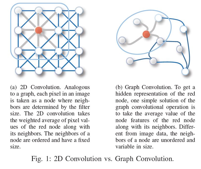
虽然深度学习技术可以捕获欧式空间数据的隐藏模式,但是目前很多应用是基于图的,这是非欧空间的数据。图数据的复杂性给现有的技术带来了很大的挑战。这是因为图数据可以是不规则的,一个图可能有不同数量的无序结点,一个结点可能有不同数量的邻接结点。这会使得一些基本操作,比如卷积,在图领域无法很好的捕获特征。除此之外,目前机器学习算法有一个重要的假设,就是假设各个结点是相互独立的,然而,图中存在很多复杂的连接信息,主要用来表征结点间的互相关性。为了解决以上问题,衍生了很多图神经网络技术。举个例子,比如,图卷积。下图对比了传统的2D卷积和图卷积。二者最大的区别在于邻接结点,一个有序一个无序,一个尺寸固定一个尺寸可变。
2.背景和定义
A. 背景
Graph neural networks vs network embedding
The main distinction between GNNs and network embedding is that GNNs are a group of neural network models which are designed for various tasks while network embedding covers various kinds of methods targeting the same task.
Graph neural networks vs graph kernel methods
The difference is that this mapping function of graph kernel methods is deterministic rather than learnable.
GNNs are much more efficient than graph kernel methods.
B. 定义
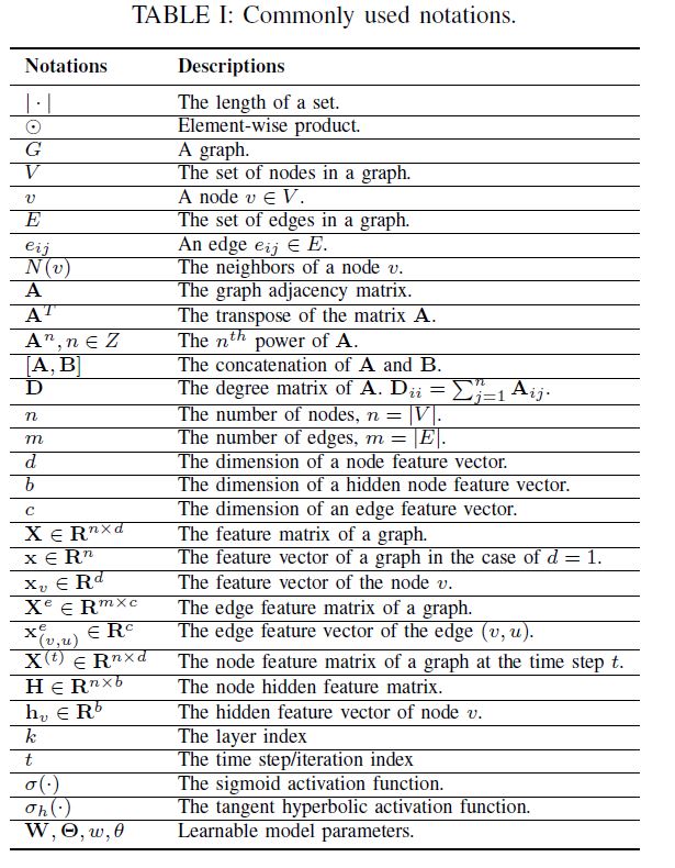
上表为本文的notation。
1.图
$ {G}=(V,E) $表示一个图。$N(v)=\{u\in V|(v,u)\in E\}$表示结点$v$的邻接结点。$\textbf{A}$是邻接矩阵,如果$A_{ij}=1$,那么表示$e_{ij}\in E$;如果$A_{ij}=0$,那么表示$e_{ij} \notin E$。$\textbf{X} \in \mathbb{R}^{n \times d} $是结点特征矩阵,$\textbf{X}^{e} \in \mathbb{R}^{m \times c}$是边特征矩阵。
2.有向图
A graph is undirected if and only if the adjacency matrix is symmetric.
3.时空图
A spatial-temporal graph is an attributed graph where the node attributes change dynamically over time.
$G^{(t)}=(V,E,\textbf{X}^{(t)}),\textbf{X}^{(t)} \in \mathbb{R}^{n \times d}$
3.分类和框架
3.1 GNN分类
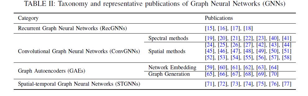
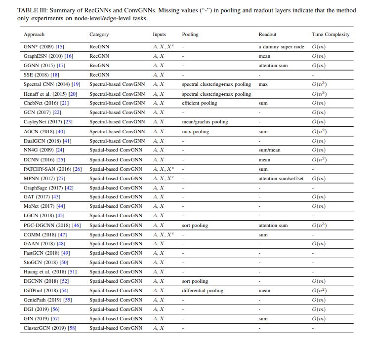
作者把GNN分成以下4类,分别为RecGNNs,ConvGNNs , GAEs, STGNNs。
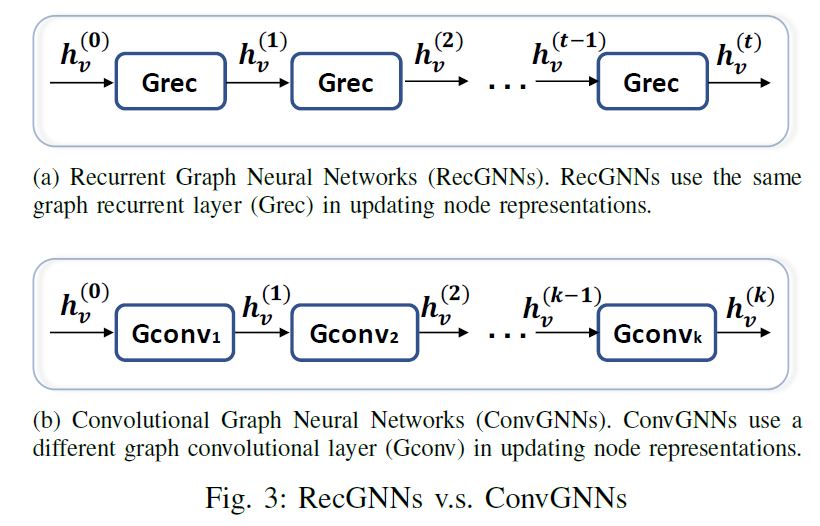
RecGNNs(Recurrent graph neural networks)
RecGNNs aim to learn node representations with recurrent neural architectures. They assume a node in a graph constantly exchanges information message with its neighbors until a stable equilibrium is reached.
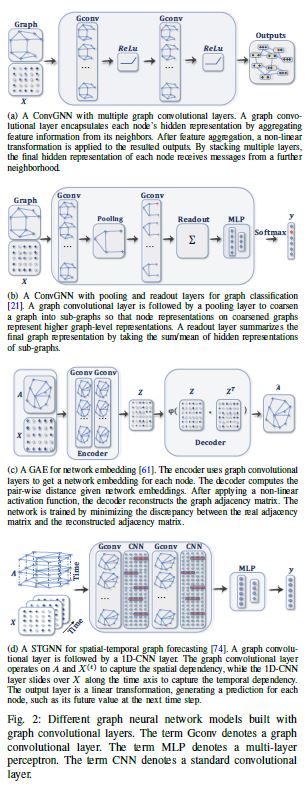
ConvGNNs(Convolutional graph neural networks )
The main idea is to generate a node $v$’s representation by aggregating its own features $\textbf{x}_v$ and neighbors’ features $\textbf{x}_u,u\in N(v)$。Different from RecGNNs, ConvGNNs stack multiple graph convolutional layers to extract high-level node representations.
GAEs(Graph autoencoders)
are unsupervised learning frameworks which encode nodes/graphs into a latent vector space and reconstruct graph data from the encoded information. GAEs are used to learn network embeddings and
graph generative distributions.
STGNNs(Spatial-temporal graph neural networks)
aim to learn hidden patterns from spatial-temporal graphs. The key idea of STGNNs is to consider spatial dependency and temporal dependency at the same time.
3.2 框架
With the graph structure and node content information as inputs, the outputs of GNNs can focus on different graph analytics tasks with one of the following mechanisms:
Node-level outputs relate to node regression and node classification tasks.
Edge-level outputs relate to the edge classification and link prediction tasks.
Graph-level outputs relate to the graph classification task.
Training Frameworks:
1.Semi-supervised learning for node-level classification
2.Supervised learning for graph-level classification
3.Unsupervised learning for graph embedding
4.RecGNNs
RecGNNs apply the same set of parameters recurrently over nodes in a graph to extract high-level node representations. 接下来介绍几种RecGNNs 结构。
GNN*
Based on an information diffusion mechanism, GNN* updates nodes’ states by exchanging neighborhood information recurrently until a stable equilibrium is reached.
结点的hidden state is recurrently updated by
$\textbf{h}_v^0$随机初始化。$f(\cdot)$是 parametric function,must be a contraction mapping, which shrinks the distance between two points after projecting them into a latent space.
训练过程分为两步,更新结点表示和更新参数,交替进行使得loss收敛。When a convergence criterion is satisfied, the last step node hidden states are forwarded to a readout layer.
GraphESN
GraphESN使用ESN提高GNN*的训练效率。GraphESN包含encoder和output output。encoder随机初始化并且不需要训练。It implements a contractive state transition function to recurrently update node states until the global graph state reaches convergence. Afterward, the output layer is trained by taking the fixed node states as inputs.
Gated Graph Neural Networks (GGNNs)
The adavantage is that it no longer needs to constrain parameters to ensure convergence. However, the downside of training by BPTT is that it sacrifices efficiency both in time and memory.
GGNN
RecGNNs 利用GRU作为循环函数
其中$\textbf{h}_v^{(0)}=\textbf{x}_v$。
GGNN uses the back-propagation through time (BPTT) algorithm to learn the model parameters.
对于大的图不适用。
SSE
proposes a learning algorithm that is more scalable to large graphs
其中$\alpha$为超参数,$\sigma(\cdot)$为sigmoid函数。
5.ConvGNNs
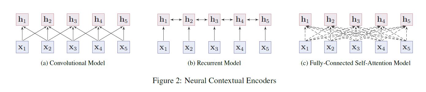
ConvGNNs与RecGNNs 主要区别在于上图。
ConvGNNs fall into two categories, spectral-based and spatial-based. Spectral based approaches define graph convolutions by introducing filters from the perspective of graph signal processing [82] where the graph convolutional operation is interpreted as removing noises from graph signals. Spatial-based approaches inherit ideas from RecGNNs to define graph convolutions by information propagation. spatial-based methods have developed rapidly recently due to its attractive efficiency, flexibility, and generality.
5.1 Spectral-based ConvGNNs
5.2 Spatial-based ConvGNNs
罗列几个基本的结构。
NN4G
其中$f(\cdot)$是激活函数,$\textbf{h}_{v}^{(0)}=0$,可以使用矩阵形式表达为:
DCNN
regards graph convolutions as a diffusion process.
其中$f(\cdot)$是激活函数。probability transition matrix $\textbf{P}\in\mathbb{R}^{n\times n},\textbf{P} = \textbf{D}^{-1}\textbf{A}$。
DCNN concatenates $\textbf{H}^{(1)},\textbf{H}^{(2)},…,\textbf{H}^{(K)}$together as the final model outputs.
PGC-DGCNN
MPNN
5.3 Graph Pooling Modules
After a GNN generates node features, we can use them for the final task. But using all these features directly can be computationally challenging, thus, a down-sampling strategy is needed. Depending on the objective and the role it plays in the network, different names are given to this strategy: (1) the pooling operation aims to reduce the size of parameters by down-sampling the nodes to generate smaller representations and thus avoid overfitting, permutation invariance, and computational complexity issues; (2) the readout operation is mainly used to generate graph-level representation based on node representations. Their mechanism is very similar. In this chapter, we use pooling to refer to all kinds of down-sampling strategies applied to GNNs.
mean/max/sum pooling is the most primitive and effective way :
$K$ is the index of the last graph convolutional layer.
some works [17], [27], [46] also use attention mechanisms to enhance the mean/sum pooling.
[101] propose the Set2Set method to generate a memory that increases with the size of the input.
还有SortPooling,DiffPool等
6.GAEs
7.STGNNs
8.APPLICATIONS
参考
https://arxiv.org/abs/1901.00596v4