import pandas as pd import pickle import os import joblib
class TrieNode(object): def __init__(self): """ Initialize your data structure here. """ self.data = {}###字母字符 self.data1={}###中文 self.is_word = False###标识是否汉字
class Trie(object):
def __init__(self): self.root = TrieNode()
def insert(self, word,word1): """ Inserts a word into the trie. :type word: str :rtype: void """ node = self.root for letter in word: child = node.data.get(letter) if not child: node.data[letter] = TrieNode() node = node.data[letter] node.is_word = True if word1 not in node.data1: node.data1[word1]=1 else: node.data1[word1]+=1
def search(self, word): """ Returns if the word is in the trie. :type word: str :rtype: bool """ node = self.root for letter in word: node = node.data.get(letter) if not node: return False return node.is_word
def starts_with(self, prefix): """ Returns if there is any word in the trie that starts with the given prefix. :type prefix: str :rtype: bool """ node = self.root for letter in prefix: node = node.data.get(letter) if not node: return False return True
def get_start(self, prefix): """ Returns words started with prefix :param prefix: :return: words (list) """ def _get_key(pre, pre_node): words_list = [] if pre_node.is_word: words_list.append([pre,pre_node.data1]) for x in pre_node.data.keys(): words_list.extend(_get_key(pre + str(x), pre_node.data.get(x))) return words_list
words = [] if not self.starts_with(prefix): return words # if self.search(prefix): # words.append(prefix) # return words node = self.root for letter in prefix: node = node.data.get(letter) return _get_key(prefix, node)
def find_result(self,string): result =self.get_start(string) result = sort_by_value(result[0][1]) result.reverse() return result[0] def sort_by_value(d): return sorted(d.items(), key=lambda k: k[1]) # k[1] 取到字典的值。
def build_tree(data,save_path):
trie = Trie() for element in data.values: trie.insert(element[0], element[1]) joblib.dump(trie, save_path) return
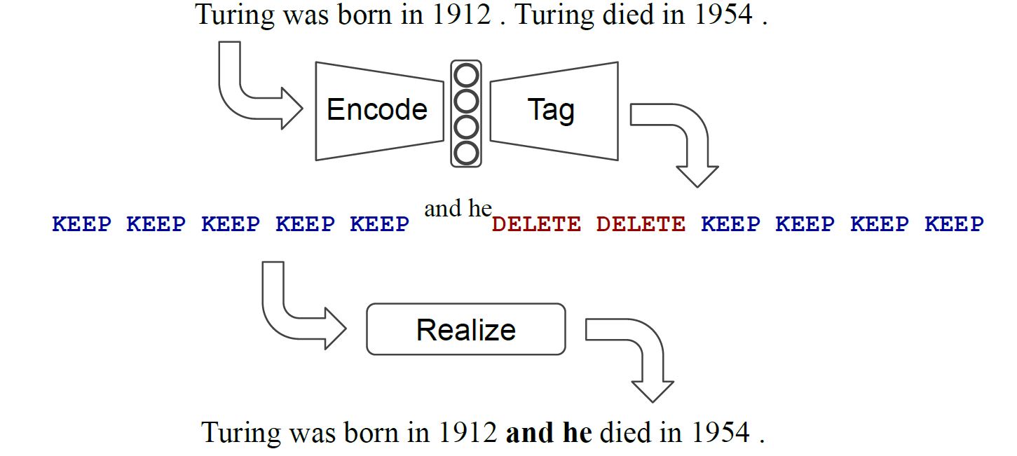
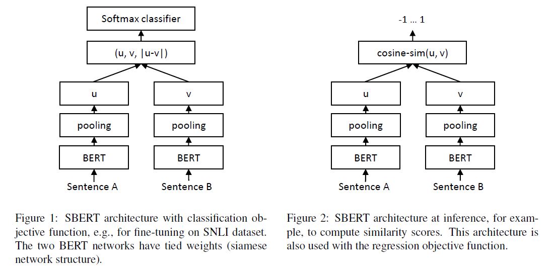
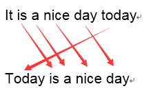
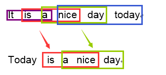
一般情况,tag分为两个大类: base tag $B$和 add tag $P$。对于base tag,就是$KEEP$或者$DELETE$当前token;对于add tag,就是要添加一个词到token前面,添加的词来源于词表$V$。实际在工程中,将$B$和$P$结合来表示,即$^{P}B$,总的tag数量大约等于$B$的数量乘以$P$的数量,即$2|V|$。对于某些任务可以引入特定的tag,比如对于句子融合,可以引入$SWAP$,如下图。
4.1.1 词表V的构建
构建目标:
最小化词汇表规模;
最大化目标词语的比例
限制词汇表的词组数量可以减少相应输出的决策量;最大化目标词语的比例可以防止模型添加无效词。
构建过程:
通过$LCS$算法(longest common sequence,最长公共子序列,注意和最长公共子串不是一回事),找出输入和输出序列的最长公共子序列,输出剩下的序列,就是需要$add$的token,添加到词表$V$,词表中的词基于词频排序,然后选择$l$个常用的。
def _compute_single_tag( self, source_token, target_token_idx, target_tokens): """Computes a single tag.
The tag may match multiple target tokens (via tag.added_phrase) so we return the next unmatched target token.
Args: source_token: The token to be tagged. target_token_idx: Index of the current target tag. target_tokens: List of all target tokens.
Returns: A tuple with (1) the computed tag and (2) the next target_token_idx. """ source_token = source_token.lower() target_token = target_tokens[target_token_idx].lower() if source_token == target_token: return tagging.Tag('KEEP'), target_token_idx + 1 # source_token!=target_token added_phrase = '' for num_added_tokens in range(1, self._max_added_phrase_length + 1): if target_token not in self._token_vocabulary: break added_phrase += (' ' if added_phrase else '') + target_token next_target_token_idx = target_token_idx + num_added_tokens if next_target_token_idx >= len(target_tokens): break target_token = target_tokens[next_target_token_idx].lower() if (source_token == target_token and added_phrase in self._phrase_vocabulary): return tagging.Tag('KEEP|' + added_phrase), next_target_token_idx + 1 return tagging.Tag('DELETE'), target_token_idx
def _compute_tags_fixed_order(self, source_tokens, target_tokens): """Computes tags when the order of sources is fixed.
Args: source_tokens: List of source tokens. target_tokens: List of tokens to be obtained via edit operations.
Returns: List of tagging.Tag objects. If the source couldn't be converted into the target via tagging, returns an empty list. """ tags = [tagging.Tag('DELETE') for _ in source_tokens] # Indices of the tokens currently being processed. source_token_idx = 0 target_token_idx = 0 while target_token_idx < len(target_tokens): tags[source_token_idx], target_token_idx = self._compute_single_tag( source_tokens[source_token_idx], target_token_idx, target_tokens) #################################################################################### # If we're adding a phrase and the previous source token(s) were deleted, # we could add the phrase before a previously deleted token and still get # the same realized output. For example: # [DELETE, DELETE, KEEP|"what is"] # and # [DELETE|"what is", DELETE, KEEP] # Would yield the same realized output. Experimentally, we noticed that # the model works better / the learning task becomes easier when phrases # are always added before the first deleted token. Also note that in the # current implementation, this way of moving the added phrase backward is # the only way a DELETE tag can have an added phrase, so sequences like # [DELETE|"What", DELETE|"is"] will never be created. if tags[source_token_idx].added_phrase: # # the learning task becomes easier when phrases are always added before the first deleted token first_deletion_idx = self._find_first_deletion_idx( source_token_idx, tags) if first_deletion_idx != source_token_idx: tags[first_deletion_idx].added_phrase = ( tags[source_token_idx].added_phrase) tags[source_token_idx].added_phrase = '' ######################################################################################## source_token_idx += 1 if source_token_idx >= len(tags): break
# If all target tokens have been consumed, we have found a conversion and # can return the tags. Note that if there are remaining source tokens, they # are already marked deleted when initializing the tag list. if target_token_idx >= len(target_tokens): # all target tokens have been consumed return tags return [] # TODO
def _compute_tags_fixed_order(self, source_tokens, target_tokens): """Computes tags when the order of sources is fixed.
Args: source_tokens: List of source tokens. target_tokens: List of tokens to be obtained via edit operations.
Returns: List of tagging.Tag objects. If the source couldn't be converted into the target via tagging, returns an empty list. """
tags = [tagging.Tag('DELETE') for _ in source_tokens] # Indices of the tokens currently being processed. source_token_idx = 0 target_token_idx = 0 while target_token_idx < len(target_tokens): tags[source_token_idx], target_token_idx = self._compute_single_tag( source_tokens[source_token_idx], target_token_idx, target_tokens) ######################################################################################### # If we're adding a phrase and the previous source token(s) were deleted, # we could add the phrase before a previously deleted token and still get # the same realized output. For example: # [DELETE, DELETE, KEEP|"what is"] # and # [DELETE|"what is", DELETE, KEEP] # Would yield the same realized output. Experimentally, we noticed that # the model works better / the learning task becomes easier when phrases # are always added before the first deleted token. Also note that in the # current implementation, this way of moving the added phrase backward is # the only way a DELETE tag can have an added phrase, so sequences like # [DELETE|"What", DELETE|"is"] will never be created. if tags[source_token_idx].added_phrase: # # the learning task becomes easier when phrases are always added before the first deleted token first_deletion_idx = self._find_first_deletion_idx( source_token_idx, tags) if first_deletion_idx != source_token_idx: tags[first_deletion_idx].added_phrase = ( tags[source_token_idx].added_phrase) tags[source_token_idx].added_phrase = '' #######################################################################################
source_token_idx += 1 if source_token_idx >= len(tags): break
# If all target tokens have been consumed, we have found a conversion and # can return the tags. Note that if there are remaining source tokens, they # are already marked deleted when initializing the tag list. if target_token_idx >= len(target_tokens): # all target tokens have been consumed return tags ####fix bug by lavine
###strategy1 added_phrase = "".join(target_tokens[target_token_idx:]) if added_phrase in self._phrase_vocabulary: tags[-1] = tagging.Tag('DELETE|' + added_phrase) print(''.join(source_tokens)) print(''.join(target_tokens)) print(str([str(tag) for tag in tags] if tags != None else None)) return tags ###strategy2 return [] # TODO
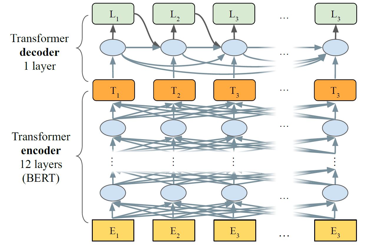
4.3 模型结构
模型主要包含两个部分:1.encoder:generates activation vectors for each element in the input sequence 2.decoder:converts encoder activations into tag labels
为了考虑标注词的关联性,decode使用了Transformer decoder,单向连接,记作$LASERTAGGER_{AR}$,这种encoder和decoder的组合的有点像BERT结合GPT的感觉decoder 和encoder在以下方面交流:(i) through a full attention over the sequence of encoder activations (ii) by directly consuming the encoder activation at the current step
Exact score :percentage of exactly correctly predicted fusions(类似accuracy)
SARI :average F1 scores of the added, kept, and deleted n-grams
2 Split and Rephrase
SARI
3 Abstractive Summarization
ROUGE-L
4 Grammatical Error Correction (GEC)
precision and recall, F0:5
七.实验结果
baseline: based on Transformer where both the encoder and decoder replicate the $BERT_{base}$ architecture
速度:1.$LASERTAGGER_{AR} $is already 10x faster than comparable-in-accuracy $SEQ2SEQ_{BERT}$ baseline. This difference is due to the former model using a 1-layer decoder (instead of 12 layers) and no encoder-decoder cross attention. 2.$LASERTAGGER_{FF}$ is more than 100x faster
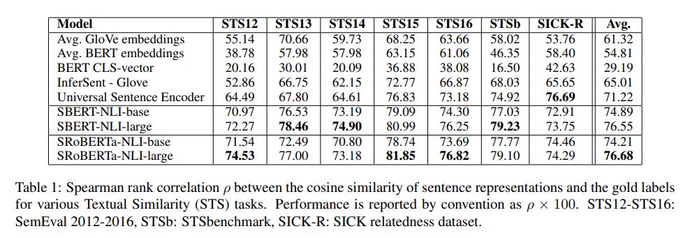
1.Using the output of the CLS-token 2.computing the mean of all output vectors (MEAN_strategy) 3.computing a max-over-time of the output vectors (MAX_strategy). The default configuration is MEAN.
from sentence_bert.sentence_transformers import SentenceTransformer, util
###load model model = SentenceTransformer(model_path)
# Single list of sentences sentences = ['The cat sits outside', 'A man is playing guitar', 'I love pasta', 'The new movie is awesome', 'The cat plays in the garden', 'A woman watches TV', 'The new movie is so great', 'Do you like pizza?']
#Compute cosine-similarities for each sentence with each other sentence cosine_scores = util.pytorch_cos_sim(embeddings, embeddings)
#Find the pairs with the highest cosine similarity scores pairs = [] for i in range(len(cosine_scores)-1): for j in range(i+1, len(cosine_scores)): pairs.append({'index': [i, j], 'score': cosine_scores[i][j]})
#Sort scores in decreasing order pairs = sorted(pairs, key=lambda x: x['score'], reverse=True)
for pair in pairs[0:10]: i, j = pair['index'] print("{} \t\t {} \t\t Score: {:.4f}".format(sentences[i], sentences[j], pair['score']))
1 2 3 4 5 6 7 8 9 10 11
The new movie is awesome 		 The new movie is so great 		 Score: 0.9283
The cat sits outside 		 The cat plays in the garden 		 Score: 0.6855
I love pasta 		 Do you like pizza? 		 Score: 0.5420
I love pasta 		 The new movie is awesome 		 Score: 0.2629
I love pasta 		 The new movie is so great 		 Score: 0.2268
The new movie is awesome 		 Do you like pizza? 		 Score: 0.1885
A man is playing guitar 		 A woman watches TV 		 Score: 0.1759
The new movie is so great 		 Do you like pizza? 		 Score: 0.1615
The cat plays in the garden 		 A woman watches TV 		 Score: 0.1521
The cat sits outside 		 The new movie is awesome 		 Score: 0.1475
class Solution:
    def uniquePaths(self, m: int, n: int) -> int:
        dp = [[1]*n] + [[1]+[0] * (n-1) for _ in range(m-1)]
        #print(dp)
        for i in range(1, m):
            for j in range(1, n):
                dp[i][j] = dp[i-1][j] + dp[i][j-1]
        return dp[-1][-1]
比如5. 最长回文子串,$dp[i][j]=dp[i+1][j-1] \ and \ s[i]==s[j]$
class Solution:
    def longestPalindrome(self, s: str) -> str:
        n = len(s)
        if n < 2:
            return s

        max_len = 1
        begin = 0
        # dp[i][j] 表示 s[i..j] 是否是回文串
        dp = [[False] * n for _ in range(n)]
        for i in range(n):
            dp[i][i] = True

        # 递推开始
        # 先枚举子串长度
        for L in range(2, n + 1):
            # 枚举左边界,左边界的上限设置可以宽松一些
            for i in range(n):
                # 由 L 和 i 可以确定右边界,即 j - i + 1 = L 得
                j = L + i - 1
                # 如果右边界越界,就可以退出当前循环
                if j >= n:
                    break

                if s[i] != s[j]:
                    dp[i][j] = False
                else:
                    if j - i < 3:
                        dp[i][j] = True
                    else:
                        dp[i][j] = dp[i + 1][j - 1]

                # 只要 dp[i][L] == true 成立,就表示子串 s[i..L] 是回文,此时记录回文长度和起始位置
                if dp[i][j] and j - i + 1 > max_len:
                    max_len = j - i + 1
                    begin = i
        return s[begin:begin + max_len]
Usually, the state of DP can use limited variables to represent such a dp[i] , dp[i] [j] ,dp[i] [j] [k].
However, sometimes, the states of a DP problem may contain multiple statuses. In this case, we can think about using the state compression approaches to represent the DP state.